Comparing groups
Written by Mohammed Saqr and Sonsoles López-Pernas
Source:vignettes/group-comparison.Rmd
group-comparison.RmdGroups of learners, conditions, or courses can differ in the order of their actions: one group may move from discussion to consensus where another moves from discussion to planning. A lag sequential model fitted to each group describes its transitions, but two models estimated separately almost always look different, if only because of sampling variation. The question a group comparison answers is whether a difference in a transition, or in the transition structure as a whole, is larger than would arise if group membership carried no information about the sequences.
lagdynamics answers it in two steps.
lsa(data, group = ) fits one model per group in a shared
state space, so the groups can be compared cell by cell even when one
group never visits a state. compare_lsa() then tests the
differences by permuting group labels over whole sequences, and
bayes_compare_lsa() gives the Bayesian counterpart, a
credible interval for each difference in transition probability.
Data
group_regulation_long is a long event log of
collaborative regulation actions, one row per action: 27,533 actions.
Two achievement groups contribute about equally: 13,721 actions from
high achievers and 13,812 from low achievers.
-
Actor:
Actoridentifies the person whose actions form one sequence. -
Action:
Action, the coded regulation action (9 states:adapt,cohesion,consensus,coregulate,discuss,emotion,monitor,plan,synthesis). -
Time:
Time, the timestamp that orders the actions; a gap of more than 900 seconds (the defaulttime_threshold) starts a new sequence. -
Group:
Achiever,HighorLow.
Group and Course are further metadata and
are not used here.
library(lagdynamics)
head(group_regulation_long)
#>   Actor Achiever Group Course                Time    Action
#> 1     1     High     1      A 2025-01-01 08:27:07  cohesion
#> 2     1     High     1      A 2025-01-01 08:35:20 consensus
#> 3     1     High     1      A 2025-01-01 08:42:18   discuss
#> 4     1     High     1      A 2025-01-01 08:50:00 synthesis
#> 5     1     High     1      A 2025-01-01 08:52:25     adapt
#> 6     1     High     1      A 2025-01-01 08:57:31 consensus
One model per group
Naming the grouping column in group fits one model per
group under the same state labels, engine, and lag.
gfit <- lsa(group_regulation_long, actor = "Actor", action = "Action",
            time = "Time", group = "Achiever")
gfit
#> <lsa_group>
#>   engine:    classical
#>   states:    9 (adapt, cohesion, consensus, coregulate, discuss, emotion, monitor, plan, synthesis)
#>   groups:    2
#>     - High:        1000 sequences
#>     - Low:         1000 sequences
The log yields 1000 sequences in each group over the same 9 states, so the two models have the same cells and can be compared one transition at a time.
summary() of a grouped fit is a data frame with one row
per group.
summary(gfit)
#>   group    engine lag n_states n_sequences n_events n_transitions n_significant alpha
#> 1  High classical   1        9        1000    13721         12721            66  0.05
#> 2   Low classical   1        9        1000    13812         12812            67  0.05
#>   lrx2 lrx2_df lrx2_p   x2 x2_df x2_p
#> 1 6147      64      0 6807    64    0
#> 2 7715      64      0 9197    64    0
The two groups are of nearly equal size: 12,721 transitions among high achievers and 12,812 among low achievers. Both reject independence decisively ( and on 64 degrees of freedom), and both have most of their 81 transitions significant (66 and 67). Each group therefore has a strongly ordered process, and the comparison asks whether the order is the same.
The reading verbs work on the grouped fit and return a leading
group column. The strongest significant transitions of both
groups:
transitions(gfit, significant = TRUE, sort = "strength") |> head(8)
#>   group      from         to lag count expected   prob prob_col adj_res         p yules_q
#> 1  High   emotion   cohesion   1   505   114.05 0.3258  0.53953    40.6  0.00e+00   0.847
#> 2  High consensus  consensus   1   283   916.99 0.0834  0.08229   -28.6 3.68e-180  -0.698
#> 3  High   discuss  synthesis   1   213    46.13 0.1063  0.72696    27.1 1.79e-161   0.881
#> 4  High   discuss       plan   1    25   458.83 0.0125  0.00858   -25.1 2.35e-139  -0.934
#> 5  High consensus coregulate   1   580   254.38 0.1710  0.60797    24.8 1.21e-135   0.663
#> 6  High consensus       plan   1  1236   777.01 0.3644  0.42416    21.9 2.64e-106   0.447
#> 7  High synthesis      adapt   1    40     3.13 0.1439  0.27972    21.2 7.61e-100   0.905
#> 8  High  cohesion  consensus   1   503   253.58 0.5362  0.14626    19.1  6.28e-81   0.554
#>    kappa kappa_z   kappa_p    lift  sign significant
#> 1  0.425    37.7 6.36e-311  4.4280  over        TRUE
#> 2 -0.709   -30.1 5.36e-199  0.3086 under        TRUE
#> 3  0.613    25.5 5.39e-143  4.6169  over        TRUE
#> 4 -0.949   -26.0 3.81e-149  0.0545 under        TRUE
#> 5  0.462    24.6 9.79e-134  2.2801  over        TRUE
#> 6  0.180    19.0  3.49e-80  1.5907  over        TRUE
#> 7  0.241    19.6  1.08e-85 12.7997  over        TRUE
#> 8  0.311    17.1  1.27e-65  1.9836  over        TRUE
Sorting applies within each group, so the first rows are those of the
high achievers; the low achievers’ rows follow in the full table. Among
high achievers, emotion -> cohesion is the strongest
regularity (505 observed against 114 expected, z = 40.6, Q = 0.847),
discuss -> synthesis follows (z = 27.1), and repeating
consensus is strongly avoided (z = -28.6). Each group’s
table describes its own process; whether a transition differs between
the groups is a separate test.
A permutation test of group differences
compare_lsa() shuffles the group labels of whole
sequences, refits both models, and sets each observed difference against
the differences produced by the shuffles. Permuting whole sequences
keeps the dependence between the actions of one sequence, so only the
link between group and transition structure is tested. The compared
measure is by default the log odds ratio of each transition against all
other transitions, which does not grow with the number of transitions
observed; diff is the high-achiever value minus the
low-achiever value. Transitions with a combined count below
min_count (default 5) are left untested. The call below
draws 500 permutations, so the smallest attainable p-value is 1/501, and
adjust = "BH" corrects the per-transition p-values for
multiple comparisons with the Benjamini-Hochberg procedure. The seed is
set once, before the permutations.
set.seed(2026)
cmp <- compare_lsa(gfit, R = 500, adjust = "BH")
cmp
#> <lsa_comparison>
#>   groups:   High vs Low
#>   measure:  log_or difference (High - Low)
#>   R:        500 label permutations
#>   edges:    38 significant of 78 tested (adjust = BH)
#>   omnibus:  statistic = 79.48, p = 0.001996
Of the 81 transitions, 78 have enough observations to be tested; the
other three have a combined count below 5 and carry NA
p-values. After the Benjamini-Hochberg adjustment, 38 of the 78 differ
between the groups. The omnibus test, the sum of squared differences
over the tested transitions, has a statistic of 79.48 and p = 0.001996,
the smallest value 500 permutations can give: no relabelling of the
sequences produced a difference as large as the observed one, so the
transition structures of the two groups differ.
The omnibus test is read as a table with
what = "global".
as.data.frame(cmp, what = "global")
#>   group_a group_b statistic p_value   R
#> 1    High     Low      79.5   0.002 500
The global table has one row per pair of groups, with the statistic, its permutation p-value, and the number of permutations, the form to report alongside the per-transition results.
transitions() reads the per-transition differences.
significant = TRUE keeps the transitions whose
Benjamini-Hochberg adjusted p-value (p_adj) is below 0.05,
and sort = "strength" orders them by the absolute
difference.
transitions(cmp, significant = TRUE, sort = "strength") |> head(8)
#>         from         to log_or_a log_or_b  diff  p_perm   p_adj significant
#> 1   cohesion      adapt   -0.794   -3.921  3.13 0.00200 0.00599        TRUE
#> 2    emotion  synthesis   -1.619   -4.522  2.90 0.00200 0.00599        TRUE
#> 3       plan  synthesis   -2.145   -4.951  2.81 0.00200 0.00599        TRUE
#> 4   cohesion  synthesis   -1.355   -3.945  2.59 0.00798 0.01887        TRUE
#> 5  synthesis    monitor   -3.229   -0.975 -2.25 0.00998 0.02162        TRUE
#> 6  synthesis       plan   -0.581   -2.680  2.10 0.00200 0.00599        TRUE
#> 7      adapt coregulate   -3.146   -1.176 -1.97 0.01597 0.03278        TRUE
#> 8 coregulate      adapt    0.778   -1.077  1.85 0.00200 0.00599        TRUE
The p-values in p_adj are Benjamini-Hochberg adjusted.
The largest differences in log odds ratio concern transitions into
adapt and synthesis.
cohesion -> adapt has a log odds ratio of -0.794 among
high achievers and -3.921 among low achievers (difference 3.13, adjusted
p = 0.00599): in the low group, cohesion is followed by adaptation far
less than base rates predict, whereas in the high group the avoidance is
mild. emotion -> synthesis (2.90) and
plan -> synthesis (2.81) follow the same pattern: high
achievers reach synthesis from emotional and planning moves that low
achievers almost never convert into synthesis. In the other direction,
synthesis -> monitor (-2.25) is relatively more frequent
among low achievers.
Barrel plot
plot() draws a group barrel plot: for the most frequent
transitions, the transition probability of each group is drawn back to
back, with the result of the permutation test on each transition.
plot(cmp)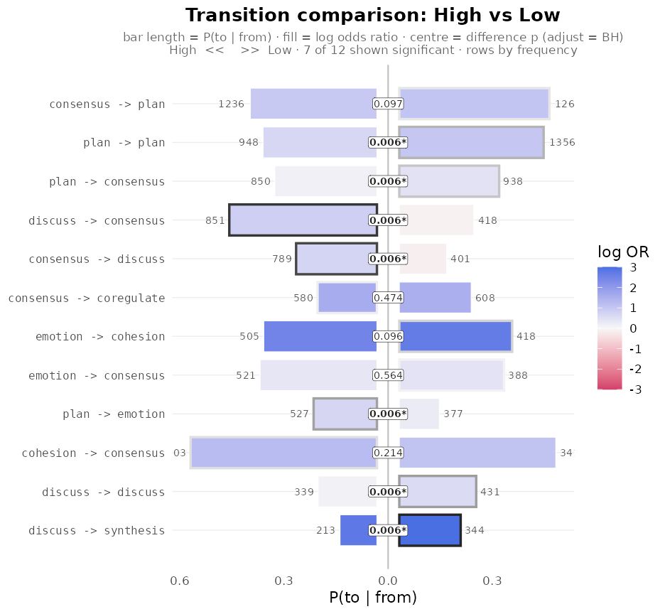
The 12 most frequent transitions are shown, ordered by frequency,
with the high achievers on the left and the low achievers on the right;
each bar is labelled with its count and the centre with the adjusted
p-value, and 7 of the 12 differ significantly. High achievers move from
discuss to consensus about twice as often as
low achievers (851 against 418 transitions) and from
consensus back to discuss likewise (789
against 401), while low achievers repeat plan more often
(1356 against 948). The most frequent transition,
consensus -> plan, does not differ (adjusted p = 0.097),
nor do emotion -> cohesion or
cohesion -> consensus: the groups share the backbone of
the process and differ in how discussion connects to consensus and
planning.
A Bayesian comparison
bayes_compare_lsa() asks a different question: given the
counts, what is the plausible range of the true difference between the
two groups’ transition probabilities? Each state’s outgoing transitions
have a Dirichlet posterior in each group, and the comparison reports the
posterior mean difference, its 95% credible interval, and the
probability of direction (pd). A transition is credibly
different when its interval excludes zero and the difference is not
negligible. No sequences are resampled, so the comparison is fast, but
it treats transitions as independent draws. adjust = "BH"
applies the Benjamini-Hochberg correction to the two-sided Bayesian
p-value (p_adj); the significant flag itself
is decided by the credible interval. seed fixes the Monte
Carlo draws.
bcmp <- bayes_compare_lsa(gfit, adjust = "BH", seed = 1)
bcmp
#> <lsa_bayes>  (Bayesian Dirichlet-Multinomial comparison)
#>   groups:    High vs Low
#>   prior:     Dirichlet(0.50)  |  draws: 10000  |  CI: 95%
#>   edges:     38 credibly different of 81 compared
transitions(bcmp, significant = TRUE, sort = "strength") |> head(8)
#>        from        to prob_a prob_b    diff  ci_low ci_high pd effect_size p_value  p_adj
#> 1   discuss consensus 0.4242 0.2143  0.2098  0.1816  0.2380  1       14.56   0e+00 0.0000
#> 2 synthesis consensus 0.5681 0.3818  0.1864  0.1092  0.2601  1        4.86   0e+00 0.0000
#> 3 synthesis     adapt 0.1434 0.2999 -0.1565 -0.2179 -0.0940  1       -4.97   0e+00 0.0000
#> 4 synthesis      plan 0.1434 0.0251  0.1183  0.0764  0.1641  1        5.30   0e+00 0.0000
#> 5 consensus   discuss 0.2324 0.1365  0.0960  0.0771  0.1153  1        9.92   0e+00 0.0000
#> 6   discuss     adapt 0.0242 0.1201 -0.0959 -0.1119 -0.0803  1      -11.77   0e+00 0.0000
#> 7      plan      plan 0.3275 0.4149 -0.0874 -0.1112 -0.0639  1       -7.21   0e+00 0.0000
#> 8  cohesion consensus 0.5342 0.4485  0.0858  0.0370  0.1328  1        3.49   8e-04 0.0024
#>   significant
#> 1        TRUE
#> 2        TRUE
#> 3        TRUE
#> 4        TRUE
#> 5        TRUE
#> 6        TRUE
#> 7        TRUE
#> 8        TRUE
The Bayesian comparison finds 38 of 81 transitions credibly
different. The largest is discuss -> consensus: a
posterior probability of 0.424 among high achievers and 0.214 among low
achievers, a difference of 0.210 with a credible interval from 0.182 to
0.238. synthesis -> consensus differs by 0.186, but its
interval (0.109 to 0.260) is wider because synthesis is a
rarely visited source state.
The two comparisons do not flag the same transitions, because they
compare different quantities. synthesis -> adapt
illustrates the difference: its posterior transition probability is
0.143 among high achievers and 0.300 among low achievers, a credible
difference of -0.16 (interval -0.218 to -0.094). The transitions with
the smallest difference in the permutation comparison are at the end of
its sorted table:
transitions(cmp, sort = "strength") |> tail(6)
#>         from        to log_or_a log_or_b    diff p_perm p_adj significant
#> 76     adapt   emotion    0.202    0.148  0.0536  0.854 0.888       FALSE
#> 77 synthesis     adapt    3.002    2.952  0.0502  0.824 0.869       FALSE
#> 78 consensus   emotion   -0.549   -0.599  0.0495  0.621 0.682       FALSE
#> 79     adapt      plan   -3.041   -3.078  0.0369  0.894 0.910       FALSE
#> 80     adapt   monitor   -0.420   -0.450  0.0307  0.926 0.926       FALSE
#> 81     adapt consensus    1.078    1.103 -0.0248  0.898 0.910       FALSE
synthesis -> adapt is among them: its log odds ratio
is 3.002 among high achievers and 2.952 among low achievers (adjusted p
= 0.869). The association between the two states, relative to their base
rates, is the same in both groups; the larger probability among low
achievers follows from a higher base rate of adapt in that
group, not from a stronger link between synthesis and adaptation. The
Bayesian comparison answers how large a difference in transition
probability is; the permutation test on the log odds ratio answers
whether the sequential association itself differs.
When to use which
-
Describe each group:
lsa(data, group = ), thensummary()andtransitions()on the grouped fit. -
Test whether groups differ, transition by transition and
overall:
compare_lsa()with an explicitadjust. It respects the dependence within sequences and can compare odds ratios, residuals, Yule’s Q, or probabilities (measure). -
Estimate how large a difference in transition probability
is:
bayes_compare_lsa(), which reports a credible interval for every difference without resampling. - More than two groups: both functions compare every pair and apply the correction across all pairs.
A difference between groups can also arise from a difference in their composition, such as the courses each group comes from; when such a confound is plausible, compare within subgroups. The checks for a single model are in Evaluating transitions, and the method itself in Lag sequential analysis.