Engines: classical, two-cell, bidirectional and dominance tests
Written by Mohammed Saqr and Sonsoles López-Pernas
Source:vignettes/articles/engines.Rmd
engines.RmdLag sequential analysis starts from one table: the counts of how often state was followed by state at a given lag. Several classical tests can be computed from that table, and they answer different questions. The classical test asks whether a directed transition occurs more or less often than the base rates of and predict (Bakeman & Quera, 2011). The two-cell test asks the same question through the odds ratio of a collapse (Bakeman & Gottman, 1997). The bidirectional test drops direction and asks whether the pair co-occurs more than expected. The two dominance tests ask whether, within the pair, outnumbers (Sackett, 1979; Wampold, 1984).
In lagdynamics each of these tests is an
engine: a function that takes the transition table and returns
per-cell statistics. Every engine is reached through
lsa(data, engine = ) or through a wrapper with the engine
fixed (lsa_classical(), lsa_two_cell(),
lsa_bidirectional(), lsa_parallel_dominance(),
lsa_nonparallel_dominance()), and every fit is read with
the same verbs: transitions(), tests(),
plot(). This guide gives, for each engine, the statistic,
the null hypothesis, the columns it adds to transitions(),
and the question it answers. It then fits all five on the same data,
shows where they agree and where they part ways, and ends with how to
register an engine of your own. The model and its reading verbs are
introduced in the LSA vignette; structural zeros,
which only the classical engine supports, are covered in the lags and structural zeros
guide.
Data
Two bundled datasets are used.
-
engagement: weekly engagement states of 138 students over 15 weeks, one row per student (wide format). States:Active,Average,Disengaged. Two rows are entirely missing, so fits use 136 sequences. With three states each table has nine cells, small enough to print in full. -
group_regulation: coded regulation actions in 2,000 collaborative learning sessions, one row per group session and one column per ordered time point (T1toT26, shorter sessions padded withNA). Nine states:adapt,cohesion,consensus,coregulate,discuss,emotion,monitor,plan,synthesis. Used to compare the engines on a larger table.
The registry lists the engines available in the session.
list_lsa_engines()
#>                    name
#> 1         bidirectional
#> 2             classical
#> 3 nonparallel_dominance
#> 4    parallel_dominance
#> 5              two_cell
#>                                                            description requires
#> 1 Sackett's bidirectional / matched-pair test on the symmetrized table
#> 2                    Bakeman & Quera classical lag sequential analysis
#> 3       Sackett's non-parallel-dominance (observed-SE + binomial) test
#> 4                      Sackett's parallel-dominance (expected-SE) test
#> 5                  2x2 cell test (odds ratio, log-OR Wald z, Yule's Q)
The five built-in engines are registered when the package loads. Any
engine added with register_lsa_engine() appears in the same
table.
Classical: adjusted residuals under independence
The classical engine tests each directed cell against sequential independence. With row totals , column totals and transitions, the expected count and the adjusted residual (Haberman, 1973) are
The null for each cell is that the next state does not depend on the current one; is referred to the standard normal. Alongside the residual, the engine reports Yule’s from the collapse of the cell (, , , ), Wampold’s unidirectional kappa with its own and (computed from event totals rather than transition totals), and the tablewise likelihood-ratio and Pearson tests with degrees of freedom. It is the only engine that supports structural zeros.
fit_classical <- lsa_classical(engagement)
fit_classical
#> Lag Sequential Analysis  -  classical  (lag 1, directed)
#>   3 states | 1734 transitions | 1870 events | 136 sequences
#>   states: Active, Average, Disengaged
#>   independence: G² = 618.3, df = 4, p <2e-16
#>
#>   Significant transitions (p < 0.05): 7 of 9
#>   strongest over-represented (of 3):
#>     Active -> Active          z =  +21.7  ***
#>     Disengaged -> Disengaged  z =  +15.4  ***
#>     Average -> Average        z =  +12.5  ***
#>
#>   Initial states:
#>     Active     0.382  ████████████████████████
#>     Average    0.368  ███████████████████████
#>     Disengaged 0.250  ████████████████
transitions(fit_classical)
#>         from         to lag count expected  prob prob_col adj_res         p yules_q
#> 1     Active     Active   1   459      247 0.698   0.7051  21.663 4.60e-104   0.828
#> 2    Average     Active   1   153      282 0.204   0.2350 -12.906  4.16e-38  -0.601
#> 3 Disengaged     Active   1    39      122 0.120   0.0599 -10.549  5.11e-26  -0.698
#> 4     Active    Average   1   176      290 0.267   0.2307 -11.319  1.06e-29  -0.534
#> 5    Average    Average   1   458      330 0.610   0.6003  12.453  1.35e-35   0.553
#> 6 Disengaged    Average   1   129      143 0.397   0.1691  -1.736  8.25e-02  -0.108
#> 7     Active Disengaged   1    23      121 0.035   0.0719 -12.557  3.64e-36  -0.826
#> 8    Average Disengaged   1   140      139 0.186   0.4375   0.176  8.60e-01   0.011
#> 9 Disengaged Disengaged   1   157       60 0.483   0.4906  15.390  1.90e-53   0.754
#>     kappa kappa_z  kappa_p  lift  sign significant
#> 1  0.4438   19.19 4.68e-82 1.858  over        TRUE
#> 2 -0.4994  -14.70 6.81e-49 0.543 under        TRUE
#> 3 -0.7069  -11.46 2.03e-30 0.320 under        TRUE
#> 4 -0.4242  -12.48 9.39e-36 0.608 under        TRUE
#> 5  0.2275    9.83 7.97e-23 1.386  over        TRUE
#> 6 -0.1618   -2.96 3.03e-03 0.902 under       FALSE
#> 7 -0.8272  -13.41 5.14e-41 0.189 under        TRUE
#> 8 -0.0903   -1.66 9.79e-02 1.010  over       FALSE
#> 9  0.3136   13.56 7.34e-42 2.618  over        TRUE
tests(fit_classical)
#>   test statistic df         p
#> 1 lrx2       618  4 1.69e-132
#> 2   x2       629  4 7.41e-135
Seven of the nine transitions depart from independence. The three
self-transitions are the over-represented cells (Active to Active,
,
459 observed against 247 expected), and every move between
Active and the other two states is under-represented. The
two transitions out of Disengaged into Average
and out of Average into Disengaged are the
only ones consistent with independence
(
and
).
The tablewise test rejects independence for the table as a whole
(,
df = 4). The answer to the classical question is that weekly engagement
is sticky: students tend to stay where they are, and direct moves
between Active and Disengaged are rare (23 and
39 transitions against expectations of 121 and 122).
Two-cell: the log odds ratio
The two-cell engine collapses each cell into the same table ( above) and tests the odds ratio with a Wald test on its logarithm:
When any of the four counts is zero, 0.5 is added to all four (the
Haldane-Anscombe correction; the amount is the engine parameter
continuity). The null is
:
being in state
does not change the odds that the next state is
.
The residual column adj_res holds this Wald
,
and the engine appends odds_ratio, log_or and
log_or_se. Kappa is not computed and there is no tablewise
test.
transitions(lsa_two_cell(engagement))
#>         from         to lag count expected  prob prob_col adj_res        p yules_q kappa
#> 1     Active     Active   1   459      247 0.698   0.7051  20.302 1.22e-91   0.828    NA
#> 2    Average     Active   1   153      282 0.204   0.2350 -12.541 4.46e-36  -0.601    NA
#> 3 Disengaged     Active   1    39      122 0.120   0.0599  -9.658 4.57e-22  -0.698    NA
#> 4     Active    Average   1   176      290 0.267   0.2307 -11.096 1.32e-28  -0.534    NA
#> 5    Average    Average   1   458      330 0.610   0.6003  12.243 1.83e-34   0.553    NA
#> 6 Disengaged    Average   1   129      143 0.397   0.1691  -1.735 8.28e-02  -0.108    NA
#> 7     Active Disengaged   1    23      121 0.035   0.0719 -10.558 4.66e-26  -0.826    NA
#> 8    Average Disengaged   1   140      139 0.186   0.4375   0.176 8.60e-01   0.011    NA
#> 9 Disengaged Disengaged   1   157       60 0.483   0.4906  14.168 1.44e-45   0.754    NA
#>   kappa_z kappa_p  lift  sign significant odds_ratio  log_or log_or_se
#> 1      NA      NA 1.858  over        TRUE     10.620  2.3627     0.116
#> 2      NA      NA 0.543 under        TRUE      0.249 -1.3896     0.111
#> 3      NA      NA 0.320 under        TRUE      0.178 -1.7283     0.179
#> 4      NA      NA 0.608 under        TRUE      0.304 -1.1901     0.107
#> 5      NA      NA 1.386  over        TRUE      3.475  1.2455     0.102
#> 6      NA      NA 0.902 under       FALSE      0.805 -0.2175     0.125
#> 7      NA      NA 0.189 under        TRUE      0.095 -2.3539     0.223
#> 8      NA      NA 1.010  over       FALSE      1.022  0.0219     0.125
#> 9      NA      NA 2.618  over        TRUE      7.144  1.9662     0.139
The two-cell test flags the same seven transitions as the classical test, with the same signs, and its Yule’s Q column is identical because both engines compute from the same collapse. The values are close but not equal (Active to Active: 20.3 against 21.7) because the Wald statistic uses the standard error of the log odds ratio rather than the expected-count variance. The engine earns its place through its effect size: an odds ratio of 10.6 for Active to Active says that an active week multiplies the odds of another active week by more than ten, and an odds ratio of 0.095 for Active to Disengaged says that an active week cuts the odds of a disengaged one by about a factor of ten.
Bidirectional: the unordered pair
The bidirectional engine asks whether two states follow each other in either order more often than expected. It symmetrises the table, , and computes adjusted residuals on with symmetric margins :
The statistic is symmetric, so the rows
and
carry the same adj_res and p; the fit is
marked undirected. A diagonal cell of
is twice the self-transition count. The engine appends
symmetric_obs
()
and symmetric_exp
();
expected also holds
.
The count, prob, lift and
sign columns are computed from the directed counts, so the
bidirectional result is read from adj_res,
symmetric_obs and symmetric_exp, not from
lift or sign.
transitions(lsa_bidirectional(engagement))
#>         from         to lag count expected  prob prob_col adj_res         p yules_q kappa
#> 1     Active     Active   1   459      494 0.698   0.7051   30.63 4.29e-206  0.8278    NA
#> 2    Average     Active   1   153      571 0.204   0.2350  -17.13  9.61e-66 -0.5675    NA
#> 3 Disengaged     Active   1    39      243 0.120   0.0599  -16.34  5.43e-60 -0.7630    NA
#> 4     Active    Average   1   176      571 0.267   0.2307  -17.13  9.61e-66 -0.5675    NA
#> 5    Average    Average   1   458      661 0.610   0.6003   17.61  2.18e-69  0.5529    NA
#> 6 Disengaged    Average   1   129      282 0.397   0.1691   -1.11  2.68e-01 -0.0489    NA
#> 7     Active Disengaged   1    23      243 0.035   0.0719  -16.34  5.43e-60 -0.7630    NA
#> 8    Average Disengaged   1   140      282 0.186   0.4375   -1.11  2.68e-01 -0.0489    NA
#> 9 Disengaged Disengaged   1   157      120 0.483   0.4906   21.76 5.10e-105  0.7544    NA
#>   kappa_z kappa_p   lift  sign significant symmetric_obs symmetric_exp
#> 1      NA      NA 0.9290 under        TRUE           918           494
#> 2      NA      NA 0.2677 under        TRUE           329           571
#> 3      NA      NA 0.1602 under        TRUE            62           243
#> 4      NA      NA 0.3080 under        TRUE           329           571
#> 5      NA      NA 0.6929 under        TRUE           916           661
#> 6      NA      NA 0.4581 under       FALSE           269           282
#> 7      NA      NA 0.0945 under        TRUE            62           243
#> 8      NA      NA 0.4972 under       FALSE           269           282
#> 9      NA      NA 1.3088  over        TRUE           314           120
The pair Active/Disengaged occurs 62 times
in either order against 243 expected
(),
and the pair Active/Average 329 times against
571
().
The pair Average/Disengaged is not
distinguishable from independence
().
The bidirectional reading agrees with the classical one but compresses
it: the classical engine needed two cells to say that
Active and Disengaged avoid each other, the
bidirectional engine says it once.
Dominance: which direction wins within a pair
The dominance engines take each pair of states and ask whether one direction outnumbers the other. Both use the difference and differ in its standard error. The parallel-dominance engine scales by the counts expected under independence,
and the non-parallel-dominance engine scales by the observed pair total,
which is the normal approximation to the exact test of
;
that exact p-value is also returned. The null is symmetry within the
pair:
and
are equally likely. The statistic is antisymmetric
()
and a self-transition has no direction, so the diagonal is
,
.
Both engines put the dominance
in adj_res and append dominance
();
the parallel engine adds dominance_se, the non-parallel
engine adds pair_totals and binomial_p. The
expected, lift and sign columns
still describe the independence model, not the dominance test.
transitions(lsa_parallel_dominance(engagement))
#>         from         to lag count expected  prob prob_col adj_res     p yules_q kappa
#> 1     Active     Active   1   459      247 0.698   0.7051   0.000 1.000   0.828    NA
#> 2    Average     Active   1   153      282 0.204   0.2350  -0.962 0.336  -0.601    NA
#> 3 Disengaged     Active   1    39      122 0.120   0.0599   1.025 0.305  -0.698    NA
#> 4     Active    Average   1   176      290 0.267   0.2307   0.962 0.336  -0.534    NA
#> 5    Average    Average   1   458      330 0.610   0.6003   0.000 1.000   0.553    NA
#> 6 Disengaged    Average   1   129      143 0.397   0.1691  -0.656 0.512  -0.108    NA
#> 7     Active Disengaged   1    23      121 0.035   0.0719  -1.025 0.305  -0.826    NA
#> 8    Average Disengaged   1   140      139 0.186   0.4375   0.656 0.512   0.011    NA
#> 9 Disengaged Disengaged   1   157       60 0.483   0.4906   0.000 1.000   0.754    NA
#>   kappa_z kappa_p  lift  sign significant dominance dominance_se
#> 1      NA      NA 1.858  over       FALSE         0         22.2
#> 2      NA      NA 0.543 under       FALSE       -23         23.9
#> 3      NA      NA 0.320 under       FALSE        16         15.6
#> 4      NA      NA 0.608 under       FALSE        23         23.9
#> 5      NA      NA 1.386  over       FALSE         0         25.7
#> 6      NA      NA 0.902 under       FALSE       -11         16.8
#> 7      NA      NA 0.189 under       FALSE       -16         15.6
#> 8      NA      NA 1.010  over       FALSE        11         16.8
#> 9      NA      NA 2.618  over       FALSE         0         11.0
No pair has a dominant direction under the parallel test. The largest
count difference is between Active and Average
(,
):
students move from Active down to Average 176
times and back up 153 times, a difference well within chance.
transitions(lsa_nonparallel_dominance(engagement))
#>         from         to lag count expected  prob prob_col adj_res      p yules_q kappa
#> 1     Active     Active   1   459      247 0.698   0.7051   0.000 1.0000   0.828    NA
#> 2    Average     Active   1   153      282 0.204   0.2350  -1.268 0.2048  -0.601    NA
#> 3 Disengaged     Active   1    39      122 0.120   0.0599   2.032 0.0422  -0.698    NA
#> 4     Active    Average   1   176      290 0.267   0.2307   1.268 0.2048  -0.534    NA
#> 5    Average    Average   1   458      330 0.610   0.6003   0.000 1.0000   0.553    NA
#> 6 Disengaged    Average   1   129      143 0.397   0.1691  -0.671 0.5024  -0.108    NA
#> 7     Active Disengaged   1    23      121 0.035   0.0719  -2.032 0.0422  -0.826    NA
#> 8    Average Disengaged   1   140      139 0.186   0.4375   0.671 0.5024   0.011    NA
#> 9 Disengaged Disengaged   1   157       60 0.483   0.4906   0.000 1.0000   0.754    NA
#>   kappa_z kappa_p  lift  sign significant dominance pair_totals binomial_p
#> 1      NA      NA 1.858  over       FALSE         0         918         NA
#> 2      NA      NA 0.543 under       FALSE       -23         329     0.2251
#> 3      NA      NA 0.320 under        TRUE        16          62     0.0559
#> 4      NA      NA 0.608 under       FALSE        23         329     0.2251
#> 5      NA      NA 1.386  over       FALSE         0         916         NA
#> 6      NA      NA 0.902 under       FALSE       -11         269     0.5421
#> 7      NA      NA 0.189 under        TRUE       -16          62     0.0559
#> 8      NA      NA 1.010  over       FALSE        11         269     0.5421
#> 9      NA      NA 2.618  over       FALSE         0         314         NA
The non-parallel test flags one pair: Disengaged to
Active outnumbers Active to
Disengaged, 39 against 23
(,
,
).
The two dominance tests differ here because the pair is rare. Under
independence the pair would occur 243 times, so the parallel standard
error is
;
it actually occurs 62 times, so the non-parallel standard error is
.
The exact binomial p-value for the same pair is 0.056, above 0.05, while
the significant column follows the normal
.
With a pair total of 62 the exact test is the one to report, and it does
not support a dominant direction: direct jumps between
Active and Disengaged run upward somewhat more
often than downward, but not reliably so.
Where the engines agree and disagree
On the larger group_regulation table the engines can be
compared on the transitions they rank first. The classical and two-cell
engines are printed first.
fit_gr <- lsa_classical(group_regulation)
transitions(fit_gr, significant = TRUE, sort = "strength") |> head(6)
#>        from         to lag count expected   prob prob_col adj_res         p yules_q
#> 1   emotion   cohesion   1   923    190.9 0.3253   0.5373    58.2  0.00e+00   0.860
#> 2   discuss  synthesis   1   557    106.8 0.1410   0.8072    48.0  0.00e+00   0.927
#> 3 synthesis      adapt   1   153     13.6 0.2347   0.2881    38.8  0.00e+00   0.904
#> 4   discuss       plan   1    46    961.6 0.0116   0.0074   -36.9 2.20e-298  -0.943
#> 5 consensus  consensus   1   519   1578.7 0.0820   0.0815   -35.5 5.32e-276  -0.661
#> 6 consensus coregulate   1  1188    519.3 0.1877   0.5671    35.3 3.36e-273   0.647
#>    kappa kappa_z   kappa_p    lift  sign significant
#> 1  0.439    55.0  0.00e+00  4.8353  over        TRUE
#> 2  0.721    46.1  0.00e+00  5.2168  over        TRUE
#> 3  0.256    37.0 2.44e-299 11.2837  over        TRUE
#> 4 -0.955   -38.2 2.88e-319  0.0478 under        TRUE
#> 5 -0.691   -37.6 7.65e-309  0.3287 under        TRUE
#> 6  0.412    34.6 5.06e-262  2.2877  over        TRUE
transitions(lsa_two_cell(group_regulation), significant = TRUE,
            sort = "strength") |> head(6)
#>        from         to lag count expected  prob prob_col adj_res         p yules_q kappa
#> 1   emotion   cohesion   1   923    190.9 0.325   0.5373    48.0  0.00e+00   0.860    NA
#> 2   discuss  synthesis   1   557    106.8 0.141   0.8072    33.3 1.08e-243   0.927    NA
#> 3 consensus coregulate   1  1188    519.3 0.188   0.5671    32.9 6.20e-237   0.647    NA
#> 4 consensus  consensus   1   519   1578.7 0.082   0.0815   -32.8 1.73e-236  -0.661    NA
#> 5 consensus       plan   1  2505   1540.3 0.396   0.4031    31.9 1.49e-223   0.465    NA
#> 6 synthesis      adapt   1   153     13.6 0.235   0.2881    28.2 3.83e-175   0.904    NA
#>   kappa_z kappa_p   lift  sign significant odds_ratio log_or log_or_se
#> 1      NA      NA  4.835  over        TRUE     13.285   2.59    0.0539
#> 2      NA      NA  5.217  over        TRUE     26.467   3.28    0.0983
#> 3      NA      NA  2.288  over        TRUE      4.662   1.54    0.0468
#> 4      NA      NA  0.329 under        TRUE      0.204  -1.59    0.0484
#> 5      NA      NA  1.626  over        TRUE      2.737   1.01    0.0315
#> 6      NA      NA 11.284  over        TRUE     19.876   2.99    0.1060
Both engines rank emotion -> cohesion first
(classical
,
two-cell
)
and agree on the sign of every listed cell, but their orderings differ
below the top: the classical engine puts
synthesis -> adapt third and
discuss -> plan fourth, the two-cell engine puts
consensus -> coregulate third and
consensus -> consensus fourth. The Wald
falls furthest below the adjusted residual for the most lopsided cells:
discuss -> synthesis (odds ratio 26.5) drops from 48.0
to 33.3 and synthesis -> adapt from 38.8 to 28.2, while
consensus -> coregulate (odds ratio 4.66) moves only
from 35.3 to 32.9. The classical
is the statistic to rank by; the odds ratio is the effect size to report
next to it.
The bidirectional engine ranks pairs, so its top rows come in mirrored pairs.
transitions(lsa_bidirectional(group_regulation), significant = TRUE,
            sort = "strength") |> head(6)
#>        from        to lag count expected   prob prob_col adj_res p yules_q kappa kappa_z
#> 1 consensus consensus   1   519     3157 0.0820   0.0815   -50.2 0  -0.661    NA      NA
#> 2   emotion  cohesion   1   923      375 0.3253   0.5373    42.2 0   0.648    NA      NA
#> 3  cohesion   emotion   1   196      375 0.1156   0.0707    42.2 0   0.648    NA      NA
#> 4      plan   discuss   1   418     1906 0.0679   0.1067   -41.3 0  -0.717    NA      NA
#> 5   discuss      plan   1    46     1906 0.0116   0.0074   -41.3 0  -0.717    NA      NA
#> 6      plan      plan   1  2304     2997 0.3742   0.3708    38.8 0   0.406    NA      NA
#>   kappa_p   lift  sign significant symmetric_obs symmetric_exp
#> 1      NA 0.1644 under        TRUE          1038          3157
#> 2      NA 2.4621  over        TRUE          1119           375
#> 3      NA 0.5228 under        TRUE          1119           375
#> 4      NA 0.2193 under        TRUE           464          1906
#> 5      NA 0.0241 under        TRUE           464          1906
#> 6      NA 0.7688 under        TRUE          4608          2997
The strongest bidirectional result is a self-transition:
consensus follows itself far less often than independence
predicts
().
The pair emotion/cohesion follows
(),
with 923 transitions one way and 196 the other. The pair
plan/discuss is avoided in both directions
().
The bidirectional view hides the fact that
emotion -> cohesion is the dominant direction of the
pair, which is the question the dominance engines answer.
transitions(lsa_parallel_dominance(group_regulation), direction = "over",
            sort = "strength") |> head(5)
#>        from         to lag count expected  prob prob_col adj_res         p yules_q kappa
#> 1   emotion   cohesion   1   923    190.9 0.325    0.537    37.5 1.59e-308   0.860    NA
#> 2   discuss  synthesis   1   557    106.8 0.141    0.807    35.9 5.32e-282   0.927    NA
#> 3 synthesis      adapt   1   153     13.6 0.235    0.288    29.3 2.17e-188   0.904    NA
#> 4 consensus coregulate   1  1188    519.3 0.188    0.567    29.0 2.53e-185   0.647    NA
#> 5  cohesion  consensus   1   844    422.8 0.498    0.133    25.7 3.65e-146   0.534    NA
#>   kappa_z kappa_p  lift sign significant dominance dominance_se
#> 1      NA      NA  4.84 over        TRUE       727        19.36
#> 2      NA      NA  5.22 over        TRUE       516        14.38
#> 3      NA      NA 11.28 over        TRUE       153         5.23
#> 4      NA      NA  2.29 over        TRUE       923        31.79
#> 5      NA      NA  2.00 over        TRUE       750        29.13
transitions(lsa_nonparallel_dominance(group_regulation), direction = "over",
            sort = "strength") |> head(5)
#>        from         to lag count expected  prob prob_col adj_res         p yules_q kappa
#> 1  cohesion  consensus   1   844      423 0.498    0.133    24.5 1.97e-132   0.534    NA
#> 2 consensus coregulate   1  1188      519 0.188    0.567    24.2 1.58e-129   0.647    NA
#> 3   emotion   cohesion   1   923      191 0.325    0.537    21.7 1.00e-104   0.860    NA
#> 4   discuss  synthesis   1   557      107 0.141    0.807    21.1  7.82e-99   0.927    NA
#> 5      plan    emotion   1   904      668 0.147    0.326    18.0  1.25e-72   0.235    NA
#>   kappa_z kappa_p lift sign significant dominance pair_totals binomial_p
#> 1      NA      NA 2.00 over        TRUE       750         938  1.75e-151
#> 2      NA      NA 2.29 over        TRUE       923        1453  1.50e-139
#> 3      NA      NA 4.84 over        TRUE       727        1119  3.36e-113
#> 4      NA      NA 5.22 over        TRUE       516         598  1.07e-116
#> 5      NA      NA 1.35 over        TRUE       621        1187   5.20e-76
With direction = "over", each pair appears once, in its
dominant direction. The parallel test ranks
emotion -> cohesion first
(,
)
and the non-parallel test ranks cohesion -> consensus
first
(,
).
Both sets point the same way: the turn-taking of these groups runs from
emotion to cohesion, from cohesion to consensus, from consensus to
coregulation, and from discussion to synthesis, much more than the
reverse. The two tests disagree on order because the parallel standard
error is large for pairs that independence expects often and small for
pairs it expects rarely, which promotes
synthesis -> adapt
(,
,
all 153 transitions of the pair in one direction) to third place.
A residual heatmap of the classical fit and of the parallel-dominance fit shows the difference in what the two engines test. The classical map has its strongest cells wherever a transition is common or rare relative to the base rates; the dominance map is antisymmetric, with each over-represented cell mirrored by an under-represented one across the diagonal.
plot(fit_gr)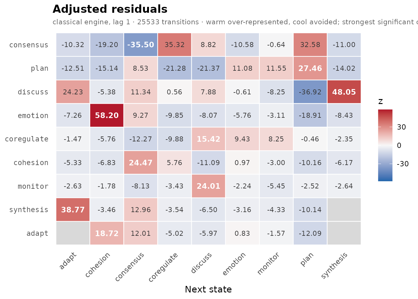
plot(lsa_parallel_dominance(group_regulation))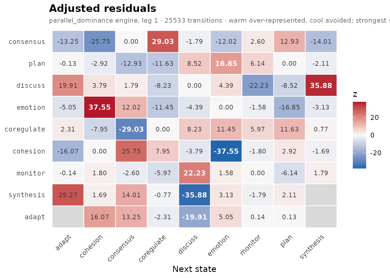
The dominance map mirrors itself:
consensus -> coregulate is
and coregulate -> consensus is
,
and the diagonal is 0. The cells that dominate are not the cells that
are most over-represented: consensus -> plan is the
fifth largest positive cell of the classical map (32.58) but only 12.93
in the dominance map, because plan -> consensus is
common too. The three grey cells in both maps are transitions with no
observed count, which the heatmap leaves blank.
Writing your own engine
The registry is open. An engine is a function that accepts
transitions (the lsa_transitions object of
counts) and ..., and returns a named list with at least the
matrices obs, exp, prob,
adj_res and p. Any further
matrix it returns becomes an extra column of transitions().
The example below defines Pearson residuals,
,
which omit the margin correction of the adjusted residual.
pearson_engine <- function(transitions, ...) {
  obs <- transitions$obs
  expected <- outer(rowSums(obs), colSums(obs)) / sum(obs)
  residual <- (obs - expected) / sqrt(expected)
  list(obs = obs, exp = expected, prob = obs / rowSums(obs),
       adj_res = residual, p = 2 * stats::pnorm(-abs(residual)))
}
register_lsa_engine("pearson", pearson_engine,
                    description = "Pearson residuals under independence")
list_lsa_engines()
#>                    name
#> 1         bidirectional
#> 2             classical
#> 3 nonparallel_dominance
#> 4    parallel_dominance
#> 5               pearson
#> 6              two_cell
#>                                                            description requires
#> 1 Sackett's bidirectional / matched-pair test on the symmetrized table
#> 2                    Bakeman & Quera classical lag sequential analysis
#> 3       Sackett's non-parallel-dominance (observed-SE + binomial) test
#> 4                      Sackett's parallel-dominance (expected-SE) test
#> 5                                 Pearson residuals under independence
#> 6                  2x2 cell test (odds ratio, log-OR Wald z, Yule's Q)
transitions(lsa(engagement, engine = "pearson"), significant = TRUE)
#>         from         to lag count expected  prob prob_col adj_res        p yules_q kappa
#> 1     Active     Active   1   459      247 0.698   0.7051   13.49 1.89e-41      NA    NA
#> 2    Average     Active   1   153      282 0.204   0.2350   -7.68 1.60e-14      NA    NA
#> 3 Disengaged     Active   1    39      122 0.120   0.0599   -7.52 5.67e-14      NA    NA
#> 4     Active    Average   1   176      290 0.267   0.2307   -6.67 2.52e-11      NA    NA
#> 5    Average    Average   1   458      330 0.610   0.6003    7.02 2.28e-12      NA    NA
#> 6     Active Disengaged   1    23      121 0.035   0.0719   -8.93 4.17e-19      NA    NA
#> 7 Disengaged Disengaged   1   157       60 0.483   0.4906   12.53 5.24e-36      NA    NA
#>   kappa_z kappa_p  lift  sign significant
#> 1      NA      NA 1.858  over        TRUE
#> 2      NA      NA 0.543 under        TRUE
#> 3      NA      NA 0.320 under        TRUE
#> 4      NA      NA 0.608 under        TRUE
#> 5      NA      NA 1.386  over        TRUE
#> 6      NA      NA 0.189 under        TRUE
#> 7      NA      NA 2.618  over        TRUE
The Pearson engine flags the same seven transitions as the classical
engine, with smaller values (Active to Active: 13.5 against 21.7),
because the adjusted residual divides by the smaller standard deviation
that accounts for the fixed margins. The Pearson residual is not
standard normal under the null and understates departures; it is shown
here as a template, not as an alternative to the classical engine.
Columns the engine did not return, such as Yule’s Q and kappa, are
NA. An engine stays registered for the session; remove it
with unregister_lsa_engine().
unregister_lsa_engine("pearson")Which engine to use
| Question | Engine | Statistic in adj_res
|
Extra columns |
|---|---|---|---|
| Does occur more or less than base rates predict? | classical |
adjusted residual | kappa, kappa_z, kappa_p; tablewise
tests |
| How large is that association, as an odds ratio? | two_cell |
Wald of |
odds_ratio, log_or,
log_or_se
|
| Do and follow each other, in either order, more than expected? | bidirectional |
adjusted residual of |
symmetric_obs, symmetric_exp
|
| Within a pair, does one direction outnumber the other? (common pairs) | parallel_dominance |
dominance, dominance_se
|
|
| The same, for rare pairs | nonparallel_dominance |
dominance, pair_totals,
binomial_p
|
The classical engine is the default and the one every inference verb
(bootstrap, permutation, group comparison) is built around; start there.
Add the two-cell engine when an effect size on the odds scale is needed
for reporting. Use the bidirectional engine when the coding does not fix
direction (two partners whose turns alternate) or when the question is
about pairing rather than sequence. Use a dominance engine when the
question is about direction within a pair, as in who leads and who
follows; prefer the non-parallel engine and its exact
binomial_p when pair totals are small. Only the classical
engine supports structural zeros (loops = FALSE or a
structural_zeros matrix); the others stop with an error of
class lagdynamics_unsupported_option.
References
Bakeman, R., & Gottman, J. M. (1997). Observing interaction: An introduction to sequential analysis (2nd ed.). Cambridge University Press.
Bakeman, R., & Quera, V. (2011). Sequential analysis and observational methods for the behavioral sciences. Cambridge University Press.
Haberman, S. J. (1973). The analysis of residuals in cross-classified tables. Biometrics, 29, 205-220.
Sackett, G. P. (1979). The lag sequential analysis of contingency and cyclicity in behavioral interaction research. In J. D. Osofsky (Ed.), Handbook of infant development (pp. 623-649). Wiley.
Wampold, B. E. (1984). Tests of dominance in sequential categorical data. Psychological Bulletin, 96(2), 424-429.