
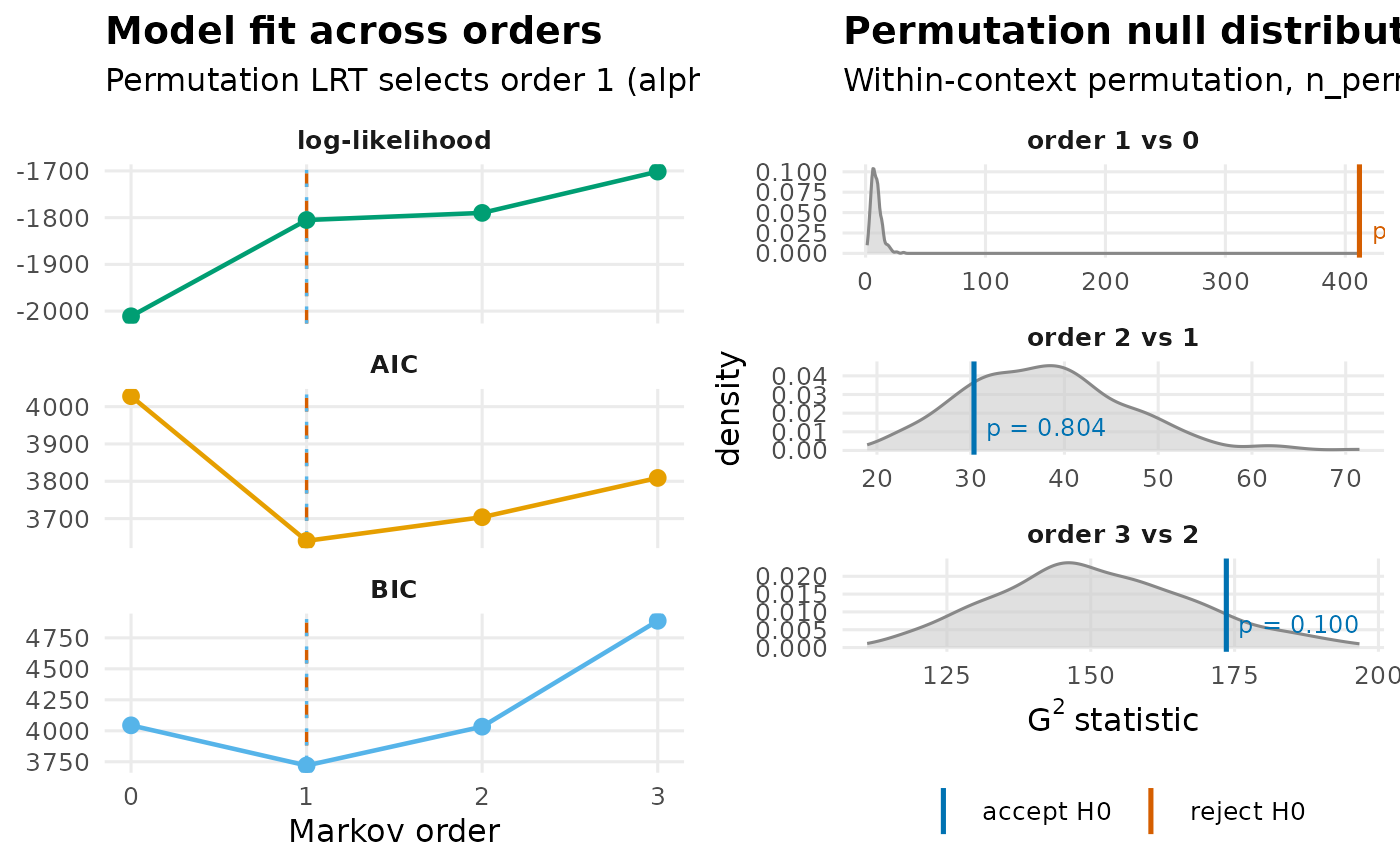
Two-panel professional visualization:
Panel A: log-likelihood, AIC, BIC across tested orders with the selected order highlighted (both the permutation-selected order and the BIC-minimizing order are marked).
Panel B: permutation null density per order with the observed \(G^2\) as a vertical marker; colored by rejection at
alpha.
Uses the Okabe-Ito colorblind-safe palette.
Arguments
- x
A
net_markov_orderobject.- panel
Which panel(s) to render:
"both","ic", or"permutation". Default"both".- combined
When
panel = "both"andcombined = TRUE(default), the two panels are drawn side-by-side. If gridExtra is installed they are arranged into a single drawable/saveable gtable (returned); otherwise basegridviewports draw both panels and a named list of the two ggplots is returned invisibly. WhenFALSE, returns that named list (ic,permutation) without drawing. Ignored whenpanel != "both".- ...
Ignored.
Value
A ggplot (single panel); for panel = "both", either a
gridExtra gtable (when gridExtra is installed) or a
named list of two ggplots (ic, permutation) drawn
side-by-side and returned invisibly.
Examples
# \donttest{
# First-order Markov data: test should select order 1
set.seed(1)
states <- letters[1:4]
tm <- matrix(runif(16), 4, 4, dimnames = list(states, states))
tm <- tm / rowSums(tm)
seqs <- lapply(1:30, function(.) {
s <- character(50); s[1] <- sample(states, 1)
for (i in 2:50) s[i] <- sample(states, 1, prob = tm[s[i - 1], ])
s
})
res <- markov_order_test(seqs, max_order = 3, n_perm = 300, seed = 1)
res$optimal_order
#> [1] 1
summary(res)
#> order loglik AIC BIC df g2 p_permutation p_asymptotic
#> 1 0 -2011.025 4028.050 4043.990 NA NA NA NA
#> 2 1 -1805.112 3640.224 3719.922 9 411.78019 0.003322259 4.193315e-83
#> 3 2 -1789.863 3703.726 4033.146 36 30.35171 0.803986711 7.337874e-01
#> 4 3 -1701.468 3808.936 4887.520 136 173.56575 0.099667774 1.633824e-02
#> significant
#> 1 NA
#> 2 TRUE
#> 3 FALSE
#> 4 FALSE
plot(res)
 # }
# }