Cluster sequences using Mixed Markov Models

Fits a mixture of Markov chains to sequence data and returns the fitted net_mmm clustering object. The fit retains assignments, posterior probabilities, mixing proportions, information criteria, and the fitted component models.

Usage

cluster_mmm(
  data,
  k = 2L,
  n_starts = 50L,
  max_iter = 200L,
  tol = 1e-06,
  smooth = 0.01,
  seed = NULL,
  covariates = NULL,
  covariate_effect = c("em", "posthoc"),
  estimator = c("auto", "firth", "multinom", "chisq"),
  cluster_by = "mmm",
  ...
)

Arguments

data: A data.frame (wide format), netobject, or tna model. For tna objects, extracts the stored data.
k: Integer. Whole finite number of mixture components, >= 2. Default: 2.
n_starts: Integer. Positive whole finite number of random restarts. Default: 50.
max_iter: Integer. Positive whole finite maximum EM iterations per start. Default: 200.
tol: Numeric. Finite positive convergence tolerance. Default: 1e-6.
smooth: Numeric. Finite non-negative Laplace smoothing constant. Default: 0.01.
seed: Integer or NULL. Random seed.
covariates: Optional. Covariates integrated into the EM algorithm to model covariate-dependent mixing proportions. Accepts a string, character vector, formula, or data.frame (same forms as build_clusters). For netobject or cograph_network input, names are resolved against $metadata first, so a typical call is build_mmm(net, k = 3, covariates = "session_label"). Unlike the post-hoc analysis in build_clusters(), these covariates directly influence cluster membership during EM estimation (see covariate_effect).
covariate_effect: How covariates enter the model. "em" (default) folds them into the EM as covariate-dependent mixing proportions, so they shape the cluster fit itself (and rows with missing covariates are dropped before fitting). "posthoc" fits a plain mixture on every sequence and uses the covariates only for the after-fit multinomial logit, so covariate values — and their missingness — never change which clusters are found. Ignored when covariates is NULL.
estimator: Multinomial fitter for the post-hoc covariate analysis (does not affect EM): "auto" (default) inspects the cluster x covariate cross-tab and falls back to "firth" only when any cell has fewer than 5 observations (separation risk), otherwise the much faster "multinom"; "firth" forces Firth's penalised likelihood via brglm2::brmultinom (finite under separation); "multinom" forces nnet::multinom (warns about separation risk); "chisq" runs descriptive tests (no logit). See build_clusters for full details.
cluster_by: Character. Accepted only as "mmm" (the default). Present so cluster_mmm() and cluster_network() share the same call shape; any other value raises an error pointing at cluster_network.
...: Unsupported. Supplying unused arguments raises an error.

Value

A fitted net_mmm clustering object. This is the same object contract returned by build_mmm. For HTNA input, its preserved actor partition is restored when the fit is materialized with build_network or Nestimate::as_htna().

Details

To materialize one network per fitted cluster, pass the result to build_network or use cluster_network(..., cluster_by = "mmm") for fitting and network construction in one call.

Examples

seqs <- data.frame(V1 = sample(c("A","B","C"), 30, TRUE),
                   V2 = sample(c("A","B","C"), 30, TRUE))
fit <- cluster_mmm(seqs, k = 2, n_starts = 1, max_iter = 10, seed = 1)
fit$assignments
#>  [1] 1 2 1 2 1 1 1 1 1 1 1 2 1 1 1 1 1 1 2 1 1 1 1 1 1 1 1 1 1 1
fit$posterior
#>             [,1]       [,2]
#>  [1,] 0.93308744 0.06691256
#>  [2,] 0.05671918 0.94328082
#>  [3,] 0.98448637 0.01551363
#>  [4,] 0.05671918 0.94328082
#>  [5,] 0.98208168 0.01791832
#>  [6,] 0.98208168 0.01791832
#>  [7,] 0.98448637 0.01551363
#>  [8,] 0.98448637 0.01551363
#>  [9,] 0.96505461 0.03494539
#> [10,] 0.98208168 0.01791832
#> [11,] 0.84431831 0.15568169
#> [12,] 0.05671918 0.94328082
#> [13,] 0.97033747 0.02966253
#> [14,] 0.98448637 0.01551363
#> [15,] 0.98448637 0.01551363
#> [16,] 0.92870181 0.07129819
#> [17,] 0.98448637 0.01551363
#> [18,] 0.98208168 0.01791832
#> [19,] 0.05671918 0.94328082
#> [20,] 0.96505461 0.03494539
#> [21,] 0.97033747 0.02966253
#> [22,] 0.97033747 0.02966253
#> [23,] 0.97033747 0.02966253
#> [24,] 0.97033747 0.02966253
#> [25,] 0.98448637 0.01551363
#> [26,] 0.97033747 0.02966253
#> [27,] 0.97033747 0.02966253
#> [28,] 0.98448637 0.01551363
#> [29,] 0.98448637 0.01551363
#> [30,] 0.98448637 0.01551363
# \donttest{
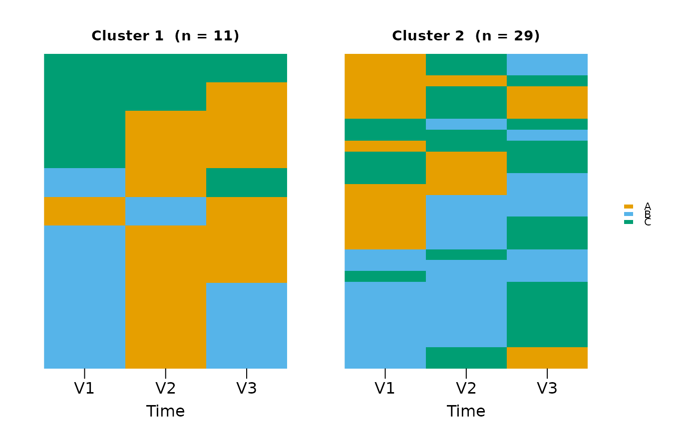
# Visualise with sequence_plot
seqs <- data.frame(
  V1 = sample(LETTERS[1:3], 40, TRUE),
  V2 = sample(LETTERS[1:3], 40, TRUE),
  V3 = sample(LETTERS[1:3], 40, TRUE)
)
fit <- cluster_mmm(seqs, k = 2)
sequence_plot(fit, type = "index")

# }

Usage

Arguments

Value

Details

See also

Examples