Comparing groups
Written by Mohammed Saqr and Sonsoles López-Pernas
Source:vignettes/comparing-groups.Rmd
comparing-groups.RmdMany questions about sequential behavior are comparative. Do high and low achievers regulate their collaboration in the same order? Do students who persist move between engagement states differently from those who drop out? Two groups can use the same states at similar rates and still differ in what follows a given history, and they can also differ in how often they reach that history at all. These are distinct questions, and a single distance between two transition matrices conflates them.
A variable-order transition tree fitted to each group gives both
pieces of information for every context: the next-state distribution
and the number of times the context occurs. The
transitiontrees package compares groups on these two axes.
The behavioral axis asks whether, given the same
context, the groups predict a different next state; it is measured per
context by the Jensen-Shannon divergence between the groups’ next-state
distributions,
where is the Shannon entropy in bits and the count of the context in group . The usage axis asks whether the groups reach the context at different rates; it is measured by a homogeneity statistic on the context’s share of each group’s positions at the same depth. The reference distribution of every statistic is built by permuting the group labels of whole sequences, and per-context p-values are adjusted for multiplicity with the Benjamini-Hochberg procedure. The model itself is introduced in the variable-order transition trees vignette.
Data
group_regulation_long is an event log of collaborative
regulation: one row per action, 27,533 rows from 2,000 students.
-
Actor:
Actoridentifies the student whose actions form a sequence. -
Time:
Timeorders the actions; a gap of more than 15 minutes starts a new sequence. -
State:
Action, one of nine regulation moves (adapt,cohesion,consensus,coregulate,discuss,emotion,monitor,plan,synthesis). -
Group:
Achiever, the student’s achievement level (HighorLow), constant within a student. -
Stratum:
Course, the course the student took (A,BorC).
Achievement and course are related. The cross-tabulation of actions
by course and achievement level shows that course A
contains only high achievers, course C only low achievers,
and course B both.
xtabs(~ Course + Achiever, data = group_regulation_long)
#>       Achiever
#> Course  High   Low
#>      A 12390     0
#>      B  1331  8295
#>      C     0  5517
Fitting one tree per group
Naming the group column in context_tree() fits one tree
per group over a shared alphabet and returns a
transitiontrees_group. The trees below hold contexts of one
action, which keeps the permutation tests fast; the collaborative
regulation case study compares deeper trees.
grp <- context_tree(group_regulation_long,
                    actor = "Actor", time = "Time", action = "Action",
                    group = "Achiever", max_depth = 1, min_count = 10)
grp
#> <transitiontrees_group>  2 groups
#>   High            10 nodes, depth <= 1, 1000 seq, 13721 obs
#>   Low             10 nodes, depth <= 1, 1000 seq, 13812 obs
summary() returns one row per group with the size and
fit of its tree.
summary(grp)
#> <transitiontrees_group summary>  2 groups
#>
#>  group n_seq n_obs n_nodes max_depth pruned logLik df  nobs   AIC   BIC perplexity
#>   High  1000 13721      10         1  FALSE -23003 80 13721 46165 46768       5.35
#>    Low  1000 13812      10         1  FALSE -23193 80 13812 46546 47148       5.36
Each group contributes 1,000 sequences and about 13,700 actions. The two trees fit their own data about equally well: a perplexity of 5.35 for high achievers and 5.36 for low achievers, against nine possible actions.
state_frequencies() lists the shares of the actions in
each group.
state_frequencies(grp)
#>    group      state count proportion
#> 1   High  consensus  3651     0.2661
#> 2   High       plan  3102     0.2261
#> 3   High    discuss  2166     0.1579
#> 4   High    emotion  1686     0.1229
#> 5   High   cohesion  1018     0.0742
#> 6   High coregulate   959     0.0699
#> 7   High    monitor   668     0.0487
#> 8   High  synthesis   316     0.0230
#> 9   High      adapt   155     0.0113
#> 10   Low       plan  3521     0.2549
#> 11   Low  consensus  3146     0.2278
#> 12   Low    discuss  2101     0.1521
#> 13   Low    emotion  1389     0.1006
#> 14   Low coregulate  1174     0.0850
#> 15   Low    monitor   848     0.0614
#> 16   Low   cohesion   821     0.0594
#> 17   Low  synthesis   413     0.0299
#> 18   Low      adapt   399     0.0289
High achievers use consensus most (26.6% of their
actions) and low achievers plan (25.5%). Low achievers use
adapt, monitor and synthesis more
often; high achievers use emotion and cohesion
more often.
Overall difference between two trees
compare_trees() tests whether two trees predict
differently overall. Its statistic is the count-weighted symmetric
Kullback-Leibler divergence between the trees’ next-state distributions,
in nats; the null distribution comes from refitting both trees after
reassigning the sequences at random to the two groups.
cmp <- compare_trees(grp, iter = 99)
summary(cmp)
#> <transitiontrees_comparison summary>
#>  distance null_mean  null_sd null_q95 p_value iter n_pathways
#>    0.0471    0.0029 0.000522  0.00367    0.01   99         10
The observed distance of 0.0471 is many times the permutation mean of 0.0029 and exceeds every one of the 99 permuted distances, so the p-value is at its floor of . The per-context breakdown shows which histories contribute most.
as.data.frame(cmp, what = "pathways")
#>       pathway count_a count_b divergence_ab divergence_ba divergence_sym
#> 1   synthesis     278     374       0.30009       0.31081        0.30545
#> 2     discuss    2003    1948       0.17777       0.20403        0.19090
#> 3    cohesion     938     757       0.11951       0.11497        0.11724
#> 4       adapt     141     368       0.04356       0.09434        0.06895
#> 5   consensus    3392    2937       0.04993       0.04583        0.04788
#> 6  coregulate     894    1076       0.04552       0.04714        0.04633
#> 7        plan    2892    3265       0.04178       0.03591        0.03884
#> 8     emotion    1550    1287       0.03462       0.03462        0.03462
#> 9     (start)   13721   13812       0.01956       0.02204        0.02080
#> 10    monitor     633     800       0.00524       0.00533        0.00529
What follows synthesis differs most between the groups
(a symmetric divergence of 0.305), then what follows
discuss (0.191) and cohesion (0.117). What
follows monitor hardly differs (0.005).
Behavioral and usage differences
compare_groups() separates the two axes, tests every
context, and works for any number of groups. summary()
reduces the result to one row with a verdict.
cg <- compare_groups(grp, iter = 99)
summary(cg)
#> Group comparison: High vs Low (10 contexts, 99 permutations)
#>   behavioral omnibus: JSD = 874.104 bits, p = 0.010
#>   usage omnibus     : G2 = 282.97, p = 0.010
#>   pathways with a behavioral difference (adjusted p < 0.05): 8
#>   pathways with a usage difference      (adjusted p < 0.05): 8
#>   pathways whose modal next state differs between groups: 4
Both omnibus tests reach the permutation floor of 0.01: given the same preceding action the groups choose different next actions, and they also reach the preceding actions at different rates. Eight of the ten contexts, the root among them, show a behavioral difference after false discovery rate adjustment, and eight of the nine contexts with a usage test (the root has none) show a usage difference.
The omnibus table and the pairwise distance are available as data frames.
as.data.frame(cg, what = "omnibus")
#>         axis                 statistic value p_value
#> 1 behavioral count-weighted JSD (bits)   874    0.01
#> 2      usage                   sum G^2   283    0.01
as.data.frame(cg, what = "distance")
#>   group_a group_b distance
#> 1    High     Low   0.0471
The behavioral statistic is the count-weighted sum of the per-context
divergences, 874 bits; the usage statistic is the sum of the per-context
values, 283. The pairwise distance is the compare_trees()
statistic, 0.0471.
The per-context table gives the counts, the modal next action in each
group, whether the modal actions differ (flips), and both
tests with raw and adjusted p-values.
as.data.frame(cg, what = "pathways")
#>       pathway depth count_total count_High count_Low modal_High modal_Low flips jsd_bits
#> 1   synthesis     1         652        278       374  consensus consensus FALSE  0.10220
#> 2     discuss     1        3951       2003      1948  consensus   discuss  TRUE  0.06557
#> 3    cohesion     1        1695        938       757  consensus consensus FALSE  0.04285
#> 4   consensus     1        6329       3392      2937       plan      plan FALSE  0.01696
#> 5  coregulate     1        1970        894      1076       plan   discuss  TRUE  0.01639
#> 6       adapt     1         509        141       368  consensus consensus FALSE  0.01536
#> 7        plan     1        6157       2892      3265       plan      plan FALSE  0.01365
#> 8     emotion     1        2837       1550      1287  consensus  cohesion  TRUE  0.01349
#> 9     (start)     0       27533      13721     13812  consensus      plan  TRUE  0.00739
#> 10    monitor     1        1433        633       800    discuss   discuss FALSE  0.00188
#>    jsd_p jsd_padj usage_g2 usage_p usage_padj
#> 1   0.01   0.0125    13.86    0.01     0.0112
#> 2   0.01   0.0125     1.43    0.21     0.2100
#> 3   0.01   0.0125    22.14    0.01     0.0112
#> 4   0.01   0.0125    47.94    0.01     0.0112
#> 5   0.01   0.0125    16.87    0.01     0.0112
#> 6   0.08   0.0889   105.31    0.01     0.0112
#> 7   0.01   0.0125    26.39    0.01     0.0112
#> 8   0.01   0.0125    29.61    0.01     0.0112
#> 9   0.01   0.0125       NA      NA         NA
#> 10  0.88   0.8800    19.42    0.01     0.0112
After discuss, high achievers most often move to
consensus and low achievers continue to
discuss. After coregulate the modal action is
plan for high achievers and discuss for low
achievers, and after emotion it is consensus
against cohesion. synthesis has the largest
behavioral divergence (0.102 bits) although both groups most often
follow it with consensus; the difference lies in the rest
of the distribution. monitor (adjusted p = 0.88) and
adapt (0.089) show no behavioral difference, and
discuss is the one context with no usage difference
(adjusted p = 0.21). adapt differs in usage
(
= 105) more than any other action but not in what follows it.
Where the groups differ
plot_difference() draws one row per context and one
column per next action. Each cell is the Pearson residual of the first
group against the no-difference null, so red cells are transitions high
achievers make more often than expected and blue cells transitions they
make less often. With comparison = cg, contexts whose
behavioral difference survives the adjustment are starred.
plot_difference(grp, comparison = cg)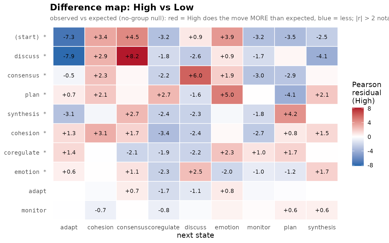
The largest residuals sit in the discuss row: after
discussing, high achievers move to consensus more often
than expected (+8.2) and to adapt less often (-7.9). High
achievers also move from consensus to discuss
(+6.0) and from plan to emotion (+5.0) more
often, and from synthesis to plan (+4.2). The
adapt and monitor rows are pale and unstarred:
what follows these actions does not differ between the groups.
Stratified permutation
The permutation tests above reassign achievement labels freely across
all students. Because course A contains only high achievers
and course C only low achievers, part of the observed
difference may be a difference between courses. Naming
Course as block restricts the permutation to
reassign labels only within each course, so the null distribution keeps
the course composition of each group fixed. The block is stored on the
fitted object, and compare_groups() uses it without further
arguments. The same argument handles repeated measures: with several
sequences per person, block set to the person column keeps
each person’s sequences together in the null.
grp_course <- context_tree(group_regulation_long,
                           actor = "Actor", time = "Time", action = "Action",
                           group = "Achiever", block = "Course",
                           max_depth = 1, min_count = 10)
cg_course <- compare_groups(grp_course, iter = 99)
summary(cg_course)
#> Group comparison: High vs Low (10 contexts, 99 stratified permutations)
#>   behavioral omnibus: JSD = 874.104 bits, p = 0.010
#>   usage omnibus     : G2 = 282.97, p = 0.010
#>   pathways with a behavioral difference (adjusted p < 0.05): 6
#>   pathways with a usage difference      (adjusted p < 0.05): 4
#>   pathways whose modal next state differs between groups: 4
The observed statistics are unchanged, and both omnibus tests remain at the permutation floor. The per-context results are more conservative: six contexts keep a behavioral difference and four a usage difference.
as.data.frame(cg_course, what = "pathways")
#>       pathway depth count_total count_High count_Low modal_High modal_Low flips jsd_bits
#> 1   synthesis     1         652        278       374  consensus consensus FALSE  0.10220
#> 2     discuss     1        3951       2003      1948  consensus   discuss  TRUE  0.06557
#> 3    cohesion     1        1695        938       757  consensus consensus FALSE  0.04285
#> 4   consensus     1        6329       3392      2937       plan      plan FALSE  0.01696
#> 5  coregulate     1        1970        894      1076       plan   discuss  TRUE  0.01639
#> 6       adapt     1         509        141       368  consensus consensus FALSE  0.01536
#> 7        plan     1        6157       2892      3265       plan      plan FALSE  0.01365
#> 8     emotion     1        2837       1550      1287  consensus  cohesion  TRUE  0.01349
#> 9     (start)     0       27533      13721     13812  consensus      plan  TRUE  0.00739
#> 10    monitor     1        1433        633       800    discuss   discuss FALSE  0.00188
#>    jsd_p jsd_padj usage_g2 usage_p usage_padj
#> 1   0.01   0.0167    13.86    0.01     0.0225
#> 2   0.01   0.0167     1.43    0.31     0.3100
#> 3   0.01   0.0167    22.14    0.13     0.1671
#> 4   0.01   0.0167    47.94    0.01     0.0225
#> 5   0.04   0.0571    16.87    0.26     0.2925
#> 6   0.24   0.2667   105.31    0.01     0.0225
#> 7   0.01   0.0167    26.39    0.04     0.0720
#> 8   0.05   0.0625    29.61    0.01     0.0225
#> 9   0.01   0.0167       NA      NA         NA
#> 10  0.45   0.4500    19.42    0.06     0.0900
coregulate and emotion, two of the contexts
whose modal next action differs between the groups, no longer pass the
behavioral adjustment (adjusted p = 0.057 and 0.062), and the usage
differences after cohesion, coregulate,
plan and monitor are no longer significant.
The behavioral differences after synthesis,
discuss, cohesion, consensus and
plan remain under a null that holds the course composition
of each group fixed.
Assumptions
- Sequences are exchangeable under the null hypothesis, within blocks
when
blockis given. - With
block, only blocks that contain more than one group contribute to the permutation; here only courseBdoes. - The tested contexts are those in the fitted trees; a context rarer
than
min_countin every group is not tested. - Weighted trees cannot be compared, because the permutation refits from the raw sequences.