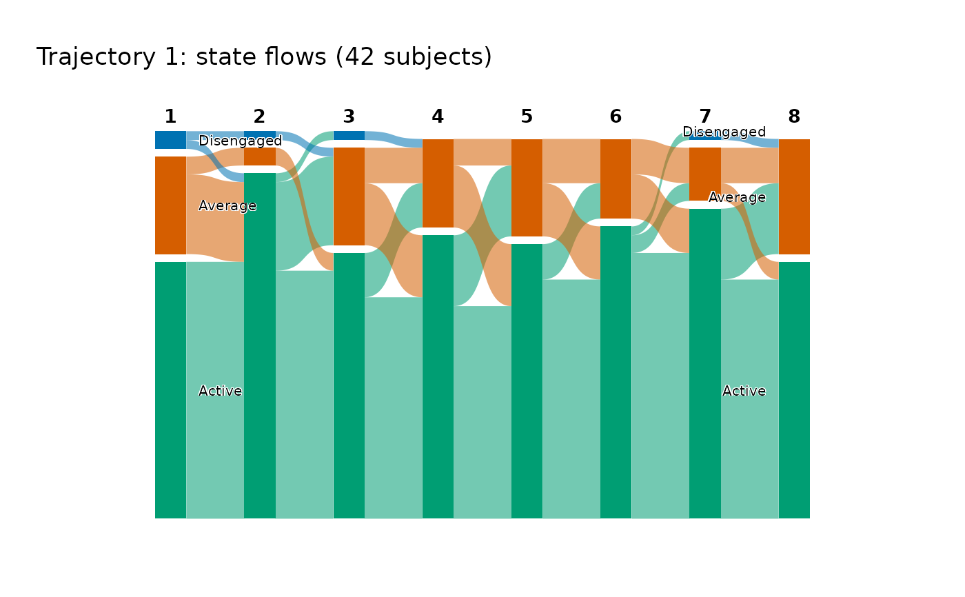
Plot State Flows Between Consecutive Time Points

Draws how subjects move between states from one time point to the next, using cograph::plot_alluvial() for aggregated bands and cograph::plot_trajectories() for individually tracked lines. Sequence index, distribution, and heatmap views remain with plot() and Nestimate; flow_plot() answers the complementary question of where movement goes, which a sequence plot ordered by similarity cannot show.

Usage

flow_plot(x, ...)

# S3 method for class 'vasstra_sequences'
flow_plot(
  x,
  type = c("alluvial", "individual"),
  colors = NULL,
  main = NULL,
  color_by = NULL,
  bundle = "auto",
  bundle_max = 50,
  ...
)

# S3 method for class 'vasstra_trajectories'
flow_plot(
  x,
  type = c("alluvial", "individual"),
  colors = NULL,
  main = NULL,
  color_by = NULL,
  bundle = "auto",
  bundle_max = 50,
  group = NULL,
  ...
)

# S3 method for class 'vasstra'
flow_plot(x, ...)

Arguments

x: A vasstra_sequences, vasstra_trajectories, or vasstra object.
...: Additional arguments passed to cograph::plot_alluvial() or cograph::plot_trajectories().
type: "alluvial" (default) for aggregated flow bands whose width is the number of subjects making that move, or "individual" for one line per subject.
colors: Optional colors, one per state, in state order. Defaults to the shared VaSSTra palette.
main: Optional plot title. A type-specific title is used by default.
color_by: State that gives a flow its color: "source" (default for "alluvial") or "destination". Individual lines also accept "first" (the default, coloring each subject by the state they start in) and "last".
bundle: Line bundling for type = "individual". "auto" (default) bundles only when subjects outnumber bundle_max lines, FALSE draws every subject, and a number sets the subjects represented by one line. Ignored by type = "alluvial".
bundle_max: Largest number of lines drawn before "auto" bundling starts. Default 50.
group: Optional trajectory label. Restricts the plot to the subjects of one trajectory, which is how a single group's movement is inspected; flow plots draw one panel and cannot be faceted.

Value

A ggplot object. Unlike the base-graphics plot() methods, which draw immediately and return their tidy data invisibly, this is returned visibly so that it prints at the console.

Details

State colors, state order, and time labels are taken from the fitted object, so a flow plot is directly comparable with the sequence heatmap and the state profiles.

Examples

# \donttest{
if (requireNamespace("cograph", quietly = TRUE)) {
  data("engagement", package = "VaSSTra")
  fit <- vasstra(
    engagement,
    state_labels = c("Disengaged", "Average", "Active")
  )
  flow_plot(fit)
  flow_plot(fit, type = "individual")
  flow_plot(fit, group = "Trajectory 1")
}
#> Using n_states = 3 to match the supplied labels.
#> Selected n_trajectories = 3 (hamming + pam, silhouette = 0.435); see `diagnostics$selection`.

# }