Magnitude difference between the frequency and probability views

Quantifies, per edge, how much row-normalization moves a transition network between its two natural summaries: raw transition counts (frequency / FTNA, build_network(method = "frequency")) and row-conditional probabilities (TNA, build_network(method = "relative")). The two matrices rank edges differently - an edge that is large in counts can be modest in probability, and a rare-source edge can dominate its row in probability. The per-edge discrepancy on a common scale is the magnitude difference.

Usage

magnitude_difference(
  data,
  actor = "Actor",
  action = "Action",
  time = NULL,
  metric = c("abs_diff", "chord_dist", "atanh_diff", "geom_norm_diff", "cv_inflation"),
  scale = c("tna_range", "rank_minmax", "minmax", "none"),
  format = c("auto", "long", "wide")
)

# S3 method for class 'magnitude_difference'
print(x, ...)

# S3 method for class 'magnitude_difference'
plot(x, type = c("stacked", "circular"), min_show = 0.01, title = NULL, ...)

Arguments

data

Long- or wide-format event log (data.frame).

actor, action, time

Column names in data (long format). time may be NULL.

metric

Discrepancy metric. One of "abs_diff" (default; absolute difference, simplest and most robust), "chord_dist" (chord distance on the unit sphere), "atanh_diff" (Fisher z-style on a bounded scale), "geom_norm_diff" (geometric-mean normalized; amplifies small edges), "cv_inflation" (per-vector SD-standardized then absolute difference).

scale

How the two weight matrices are placed on a common scale before differencing. "tna_range" (default) rescales FTNA linearly into TNA's [min, max] range and leaves TNA untouched, so the difference is in TNA probability units. "rank_minmax" converts each matrix's values to ranks scaled to [0, 1] (ordinal). "minmax" scales each matrix's raw values to [0, 1] separately (asymmetric - TNA's max and FTNA's max map to the same value despite differing native ranges). "none" uses raw weights.

format

Input format passed through to build_network(); "auto" (default) treats the data as wide when action is not a column.

x

For the print() and plot() methods: an object of class magnitude_difference.

...

In plot.magnitude_difference(): Ignored. In print.magnitude_difference(): Passed to plotting helpers (ignored by print).

type

Plot style, "stacked" (default) or "circular".

min_show

For type = "circular", drop edges whose magnitude is below this fraction of the maximum.

title

Plot title. NULL generates one from the metric and scale.

Value

An object of class "magnitude_difference": a list with $edges (per-edge data.frame with columns from, to, ftna, tna, signed = tna - ftna, and value = the chosen metric), $metric, $scale, $weights_ftna, $weights_tna, and $states.

In print.magnitude_difference(): print invisibly returns x.

In plot.magnitude_difference(): plot returns a ggplot object.

See also

build_network(), compare_model()

Examples

data(group_regulation_long, package = "Nestimate")
fit <- magnitude_difference(group_regulation_long,
                            actor = "Actor", action = "Action",
                            time = "Time")
print(fit)
#> magnitude_difference object
#>   metric: abs_diff   scale: tna_range 
#>   states (9):  adapt, cohesion, consensus, coregulate, discuss, emotion, monitor, plan, synthesis
#>   edges: 81 
#>   magnitude-difference summary (abs_diff):
#>    Min. 1st Qu.  Median    Mean 3rd Qu.    Max. 
#> 0.00000 0.01143 0.03002 0.06035 0.06894 0.42910 
# \donttest{
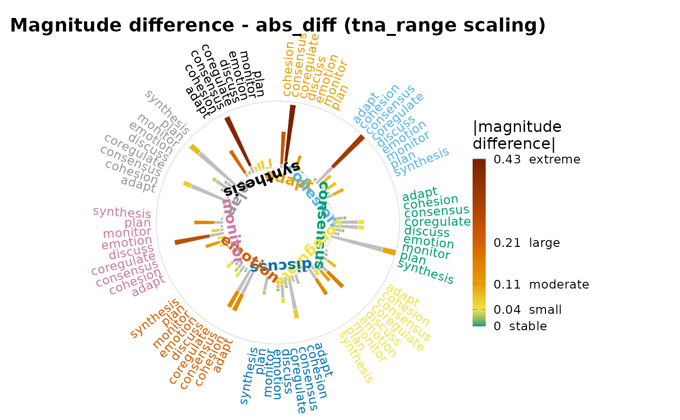
# The polar portrait shows which edges row-normalization promotes.
plot(fit)                       # stacked polar portrait

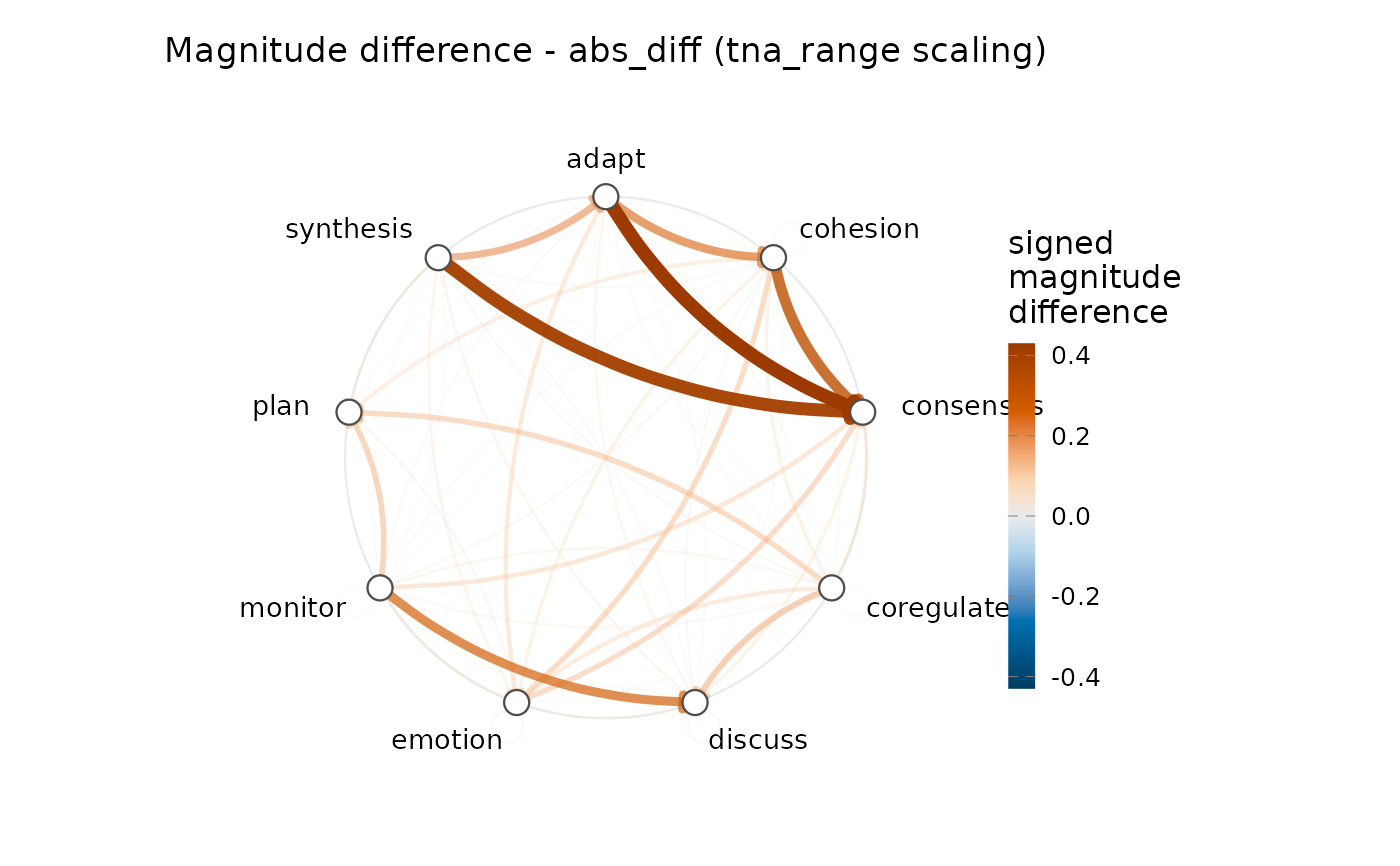
plot(fit, type = "circular")    # chord-style diagram

# }