Build HONEM Embeddings for Higher-Order Networks

Constructs low-dimensional embeddings from a Higher-Order Network (HON) that preserve higher-order dependencies. Uses exponentially-decaying matrix powers of the HON transition matrix followed by truncated SVD.

Usage

build_honem(hon, dim = 32L, max_power = 10L)

# S3 method for class 'net_honem'
print(x, ...)

# S3 method for class 'net_honem'
summary(object, ...)

# S3 method for class 'net_honem'
plot(x, dims = c(1L, 2L), ...)

Arguments

hon

A net_hon object from build_hon, or a square weighted adjacency matrix.

dim

Integer. Embedding dimension (default 32). Silently capped at n_nodes - 1; the dimension actually used is reported in the returned dim component.

max_power

Integer. Maximum walk length for neighborhood computation (default 10). Higher values capture longer-range structure.

x

For the print() and plot() methods: an object of class net_honem.

...

In plot.net_honem(): Additional arguments passed to plot. In print.net_honem() and summary.net_honem(): Additional arguments (ignored).

object

For the summary() method: an object of class net_honem.

dims

Integer vector of length 2. Dimensions to plot (default: c(1, 2)).

Value

An object of class net_honem with components:

embeddings

Numeric matrix (n_nodes x dim) of node embeddings, row names = node names, column names dim_1, dim_2, ...

nodes

Character vector of node names.

singular_values

Numeric vector of top singular values.

explained_variance

Proportion of variance explained.

dim

Embedding dimension used.

max_power

Maximum power used.

n_nodes

Number of nodes embedded.

In print.net_honem() and plot.net_honem(): The input object, invisibly.

In summary.net_honem(): A data.frame with one row per node: column node (node label) followed by dim1, dim2, ..., dimd embedding coordinates, returned visibly; the summary text is printed as a side effect.

Details

HONEM is parameter-free and scalable - no random walks, skip-gram, or hyperparameter tuning required.

References

Saebi, M., Ciampaglia, G. L., Kaplan, L. M., & Chawla, N. V. (2020). HONEM: Learning Embedding for Higher Order Networks. Big Data, 8(4), 255-269.

Examples

seqs <- list(c("A","B","C","D"), c("A","B","C","A"), c("B","C","D","A"))
hem <- build_honem(build_hon(seqs, max_order = 2), dim = 2)

# \donttest{
trajs <- list(c("A","B","C","D"), c("A","B","D","C"),
              c("B","C","D","A"), c("C","D","A","B"))
hon <- build_hon(trajs, max_order = 2)
emb <- build_honem(hon, dim = 4)
print(emb)
#> HONEM: Higher-Order Network Embedding
#>   Nodes:      4
#>   Dimensions: 3
#>   Max power:  10
#>   Variance explained: 94.6%
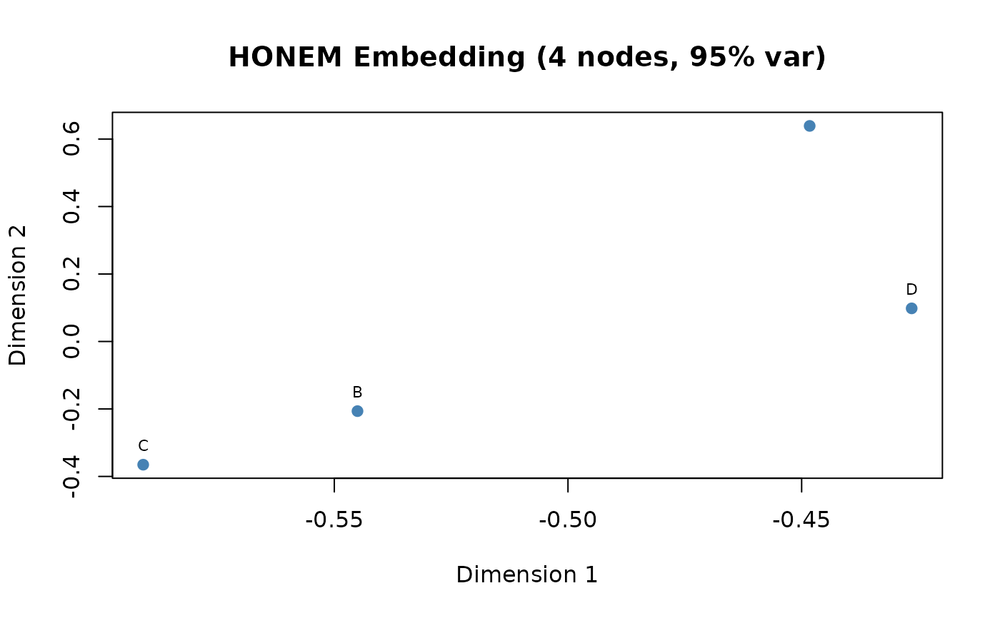
plot(emb)

# }