Comparing two networks with compare_networks()

High and low achievers in group_regulation_long are compared with a permutation test (1,000 permutations).

achievers <- build_network(group_regulation_long, method = "relative",
                           actor = "Actor", action = "Action",
                           time = "Time", group = "Achiever")
cmp <- compare_networks(achievers, test = "permutation", iter = 1000, seed = 1)
cmp

## Network comparison (permutation, iter = 1000, alpha = 0.05, adjust = none): 2 networks, 1 pairs, scaling = none
##   networks: High (9 nodes, directed), Low (9 nodes, directed)
## 
##  pair        pearson mean|diff| max|diff| largest change                    
##  High vs Low 0.92    0.03       0.21      discuss -> consensus (High higher)
##  sig edges
##  42       
## 
## Tables: summary(x), edge_differences(x), node_differences(x), global_differences(x), network_metrics(x). Plot: plot(x, type = ...)

summary(cmp)

##         pair network_a network_b n_cells n_differing share_higher_a
##  High vs Low      High       Low      81          78           0.51
##  share_higher_b mean_abs_diff max_abs_diff pearson spearman cosine jaccard
##            0.46          0.03         0.21    0.92     0.92   0.95    0.75
##              top_edge top_edge_higher n_sig_edges n_sig_nodes m_stat   m_p
##  discuss -> consensus            High          42          16   2.61 0.001
##  s_stat   s_p
##    0.21 0.001

The networks are similar overall (Pearson 0.92, cosine 0.95, Jaccard 0.75) but differ in 42 of 78 transitions and 16 of 27 node measures. The global test is significant (M = 2.61, p = 0.001).

networks

plot(cmp, type = "networks")

The two networks side by side.

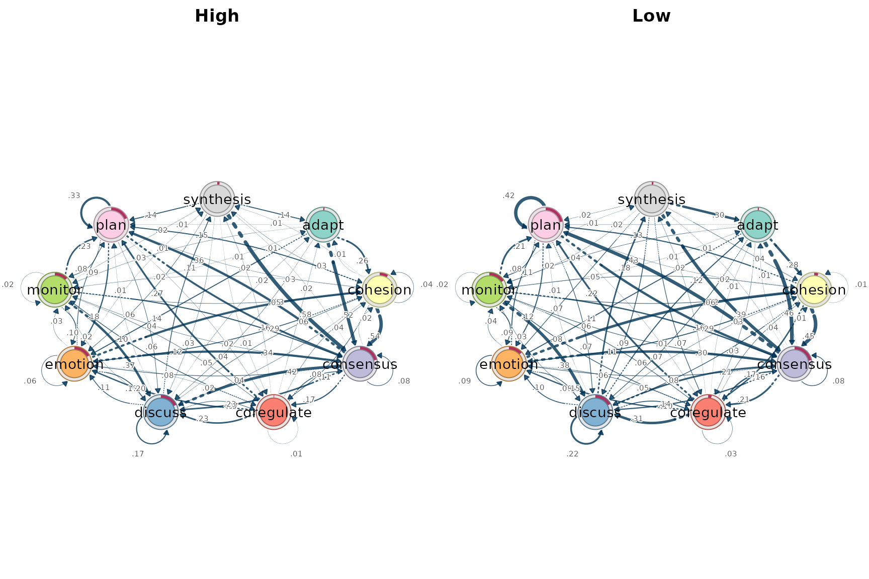
difference

plot(cmp, type = "difference")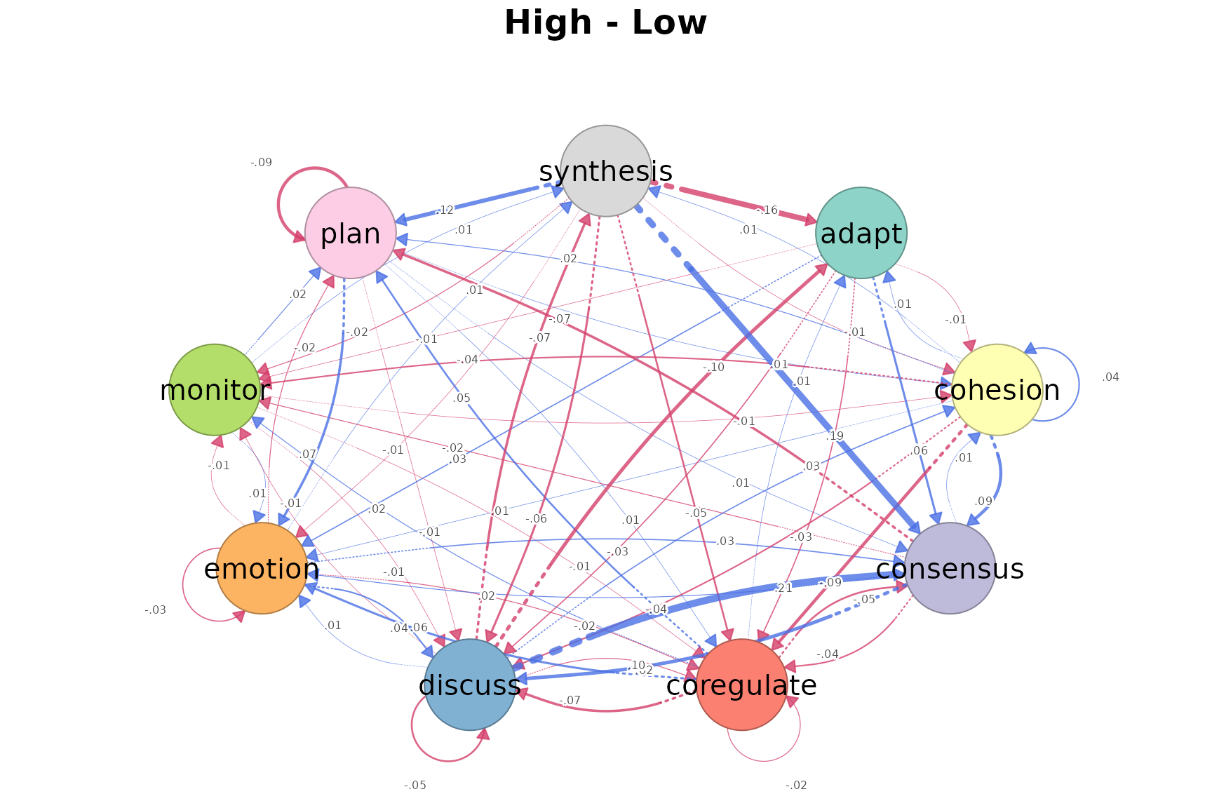

High minus Low for each transition: blue is higher in High, red higher in Low; the line style also carries the sign.

edges

plot(cmp, type = "edges")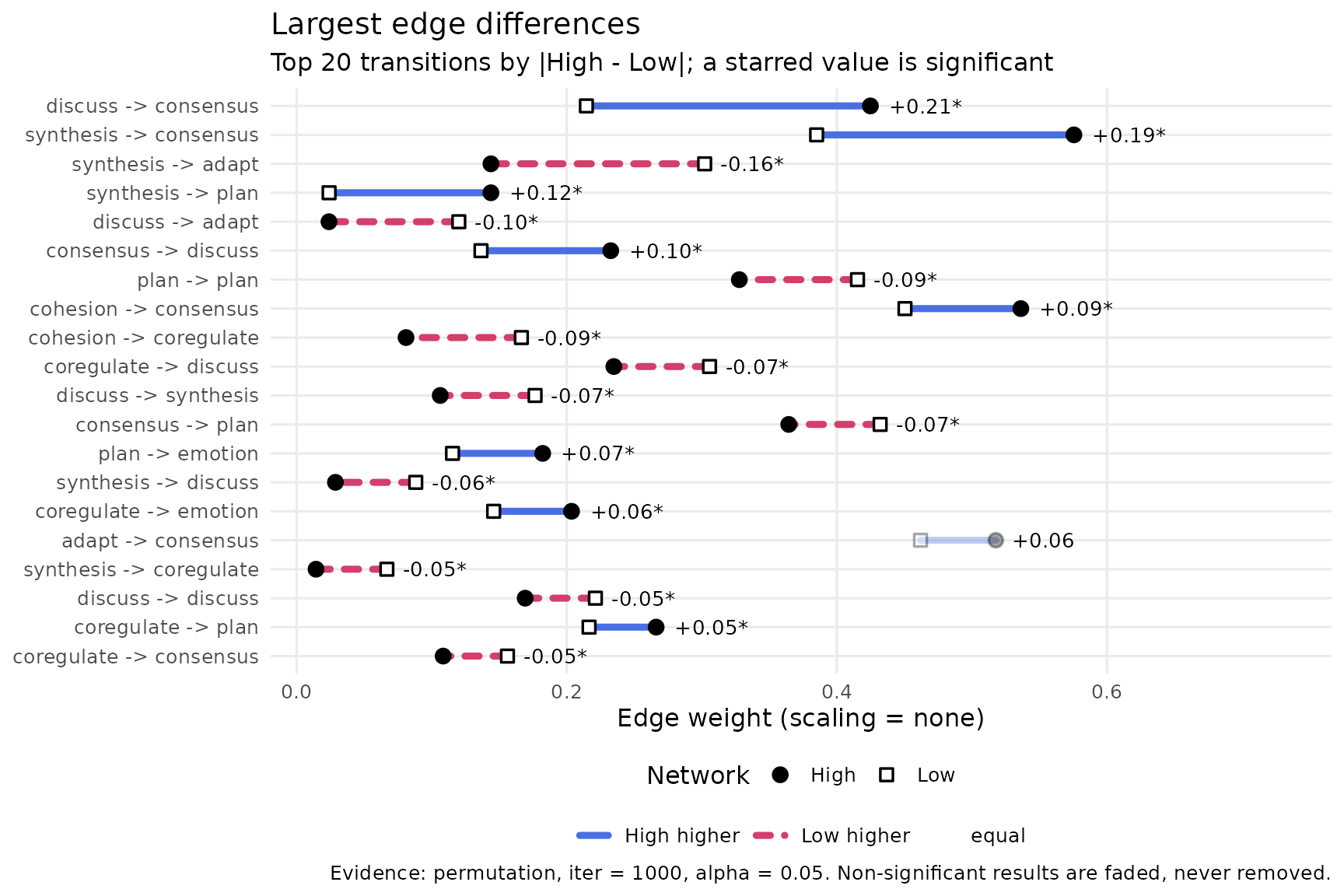

The largest differences: discuss to consensus (0.42 vs 0.21) and synthesis to consensus (0.58 vs 0.39) are higher in High; synthesis to adapt is higher in Low (0.14 vs 0.30). All have p = 0.001.

nodes

plot(cmp, type = "nodes")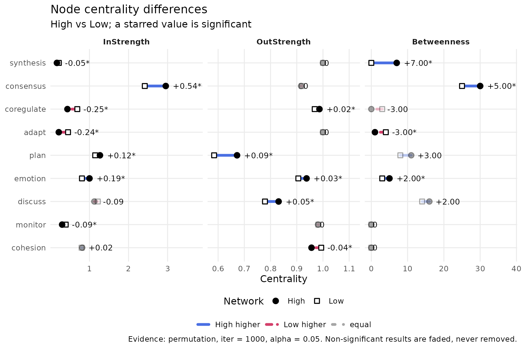

Centrality differences per state. synthesis has higher betweenness in High (7 vs 0, p = 0.003); adapt in Low (4 vs 1, p = 0.001).

global

plot(cmp, type = "global")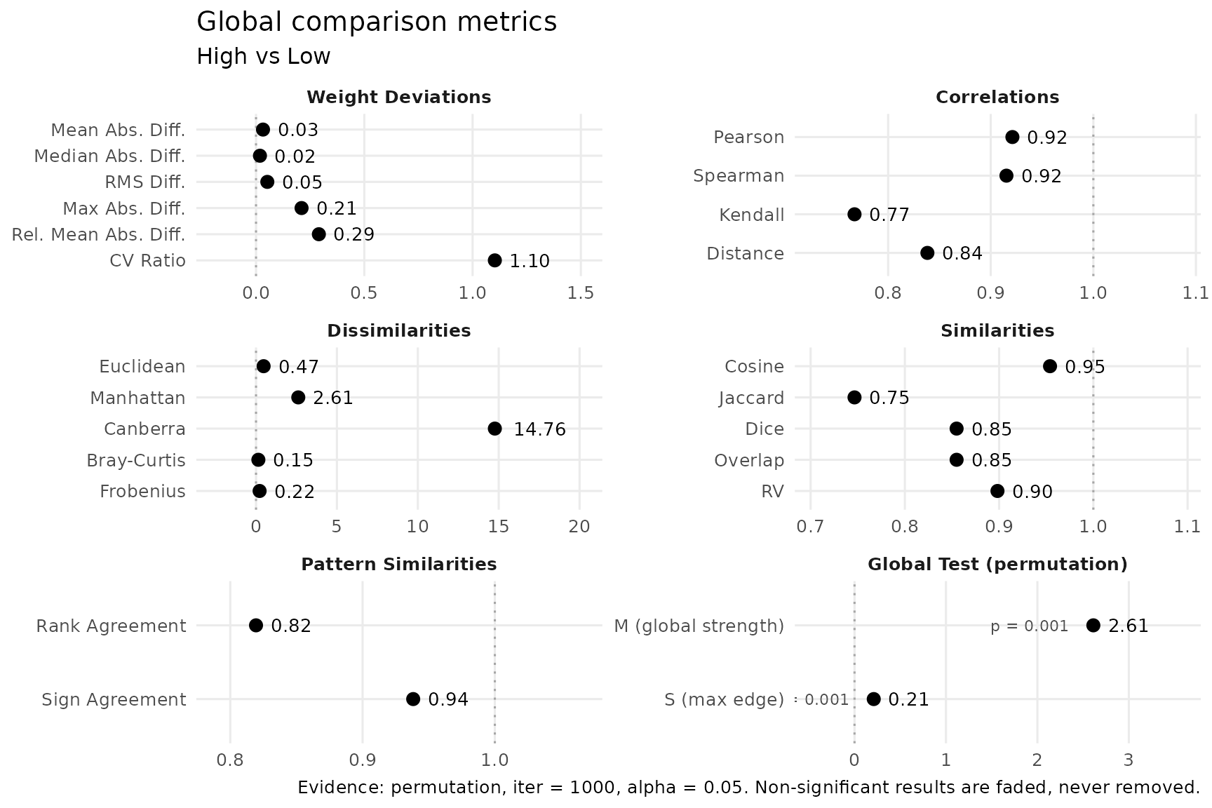

The 22 similarity and distance metrics of global_differences(cmp), grouped by category.

heatmap

plot(cmp, type = "heatmap")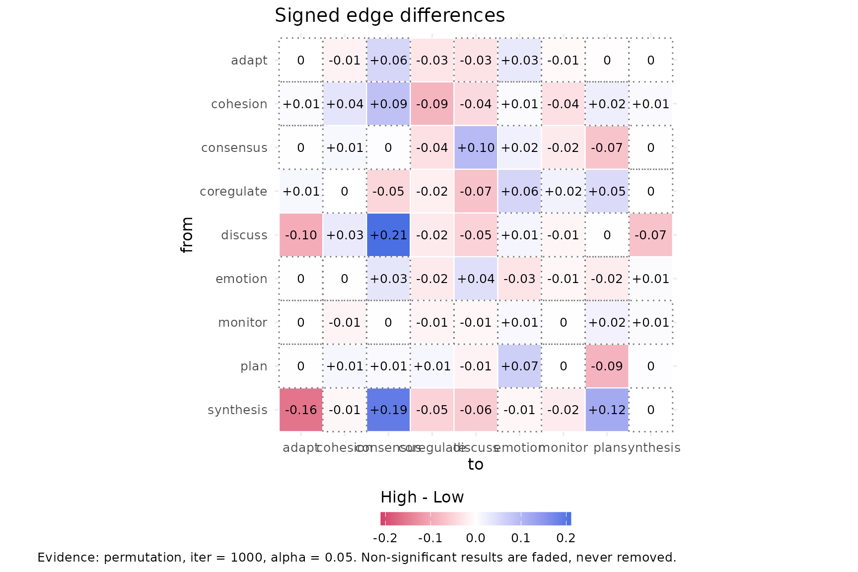

Every cell of the High minus Low difference matrix, with its value.

scatter

plot(cmp, type = "scatter")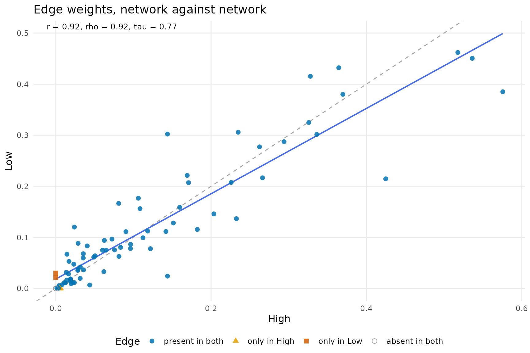

Each transition’s weight in High against Low; points on the diagonal are equal in both (Pearson 0.92).

inference

plot(cmp, type = "inference")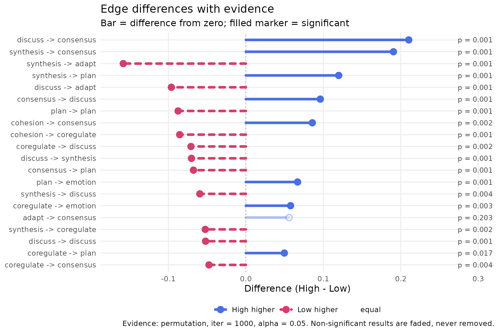

Edge differences with their permutation p-values; filled markers are significant at 0.05.

Accounting for nesting

nested <- compare_networks(achievers, test = "permutation", iter = 1000,
                           seed = 1, actor = "Group")
nested

## Network comparison (permutation, iter = 1000, alpha = 0.05, adjust = none, actor = Group): 2 networks, 1 pairs, scaling = none
##   networks: High (9 nodes, directed), Low (9 nodes, directed)
## 
##  pair        pearson mean|diff| max|diff| largest change                    
##  High vs Low 0.92    0.03       0.21      discuss -> consensus (High higher)
##  sig edges
##  42       
## 
## Tables: summary(x), edge_differences(x), node_differences(x), global_differences(x), network_metrics(x). Plot: plot(x, type = ...)

tail(global_differences(nested, digits = 3), 5)

##         pair network_a network_b                  category
##  High vs Low      High       Low Global Test (permutation)
##  High vs Low      High       Low Global Test (permutation)
##  High vs Low      High       Low                   Nesting
##  High vs Low      High       Low                   Nesting
##  High vs Low      High       Low                   Nesting
##                 metric         key  value perm_p perm_sig
##    M (global strength)      perm_M  2.612  0.001     TRUE
##           S (max edge)      perm_S  0.210  0.001     TRUE
##                    ICC         icc -0.002     NA       NA
##  Design effect (edges)  deff_edges  1.009     NA       NA
##      Design effect (M) deff_global  1.169     NA       NA

Students are nested in teams, and the achievement level is given per team. With actor = "Group", the permutation test reassigns whole teams instead of single students, and global_differences() gains three Nesting rows. The ICC is −0.002, which indicates little evidence of a nesting effect; the design effect is 1.01 for the transitions and 1.17 for M. The networks still differ overall (M = 2.61, p = 0.001), and 42 transitions remain significant.