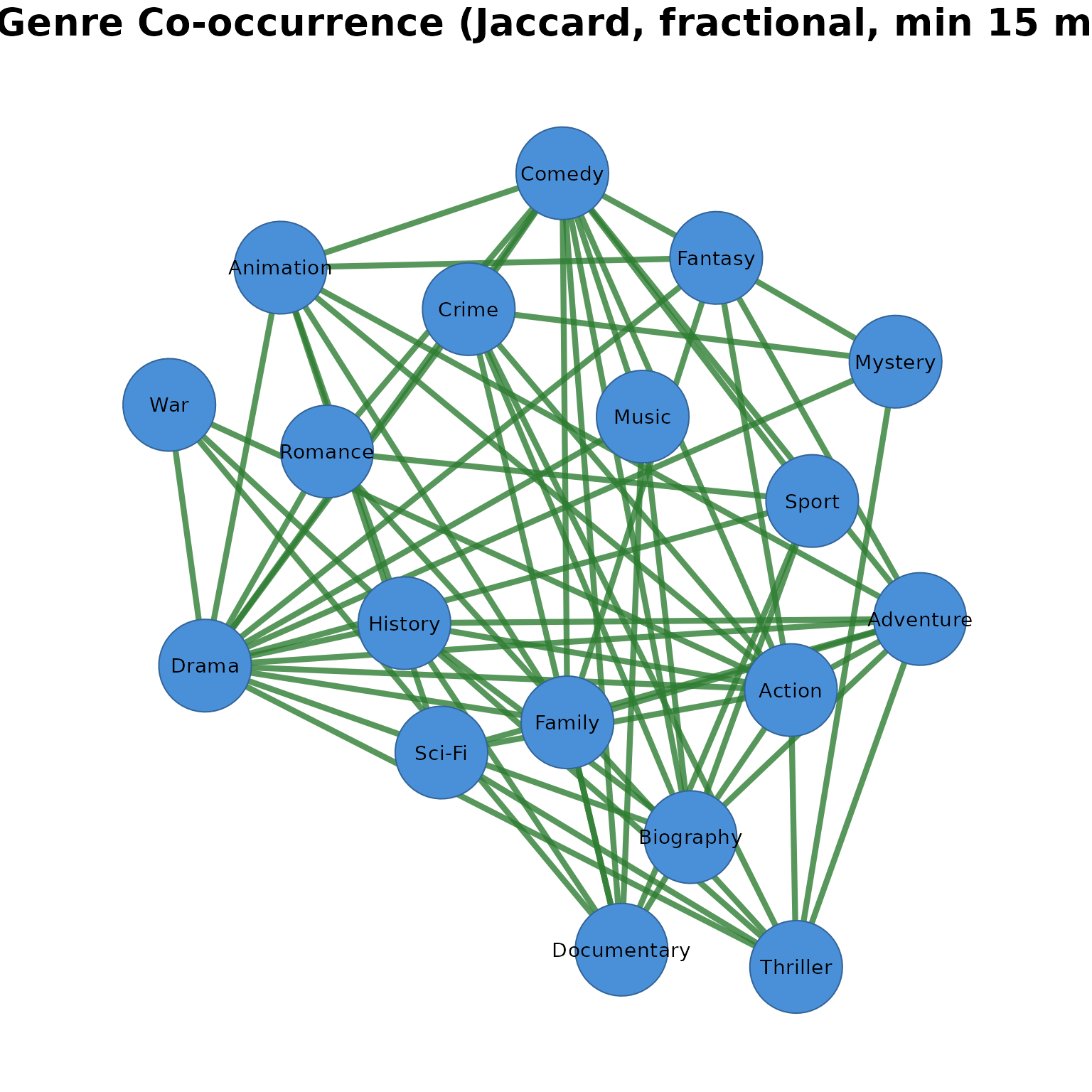
This tutorial demonstrates every feature of the cooccure
package using 1,000 highly-rated IMDB movies (rating
7.0,
1,000 votes, 1970–2024).
Starting from raw tabular data, we build genre co-occurrence
networks, construct actor collaboration networks, compare co-occurrence
patterns across decades and rating bands, apply different similarity
measures and counting methods, and export results to Gephi,
igraph, and cograph for visualization and
downstream analysis.
Data
The dataset contains the title of the movie, the year and decade, the
genres (comma-separated), the average rating, the number of
votes, and the rating band.
head(movies)
#>       tconst                          primaryTitle startYear
#> 1  tt0118117                       The War at Home      1996
#> 2 tt10534996                                 Josep      2020
#> 3  tt4686844                   The Death of Stalin      2017
#> 4  tt0089957 Samaya obayatelnaya i privlekatelnaya      1985
#> 5  tt3469964                         Blind Massage      2014
#> 6  tt7647198                       Love and Shukla      2017
#>                      genres decade averageRating numVotes
#> 1                     Drama  1990s           7.0     2733
#> 2 Animation,Biography,Drama  2020s           7.4     2340
#> 3      Comedy,Drama,History  2010s           7.3   126237
#> 4            Comedy,Romance  1980s           7.4     2521
#> 5                     Drama  2010s           7.2     1804
#> 6      Comedy,Drama,Romance  2010s           7.2     1234
1. Genre co-occurrence (delimited field)
Each movie has a comma-delimited genres column, where
genres that appear in the same movie are connected. To analyze their
co-occurrence we need to call cooccurrence and specify the
field argument specifying the column and sep
specifying the delimiter that separates values within that field.
cooccurrence(movies, field = "genres", sep = ",")
#> # cooccurrence: 22 nodes, 129 edges | density: 0.5584 | mean degree: 11.7273 | 1000 transactions
#> # similarity: none | counting: full
#> # possible edges: 231 | isolates: 0
#> # top nodes: Drama(deg=20,str=812), Comedy(deg=19,str=412), Action(deg=17,str=295), Romance(deg=17,str=237), Adventure(deg=15,str=195)
#>       from          to weight count
#>     Comedy       Drama    159   159
#>      Drama     Romance    131   131
#>      Crime       Drama     91    91
#>     Action       Drama     71    71
#>     Comedy     Romance     63    63
#>     Action       Crime     59    59
#>  Biography       Drama     59    59
#>      Drama    Thriller     57    57
#>     Action   Adventure     44    44
#>  Biography Documentary     44    44
#> # ... 119 more edges
The result shows 22 genre nodes and 129 edges. Drama dominates the top pairs simply because it is the most frequent genre, inflating co-occurrence with nearly every other genre regardless of actual association strength. Jaccard similarity normalizes for this, so the strongest edges reflect true affinity rather than frequency. A directed co-occurrence graph is then built and its degree distribution plotted as a bar chart, showing how many nodes share each degree value and whether connectivity is concentrated or evenly spread across genres.
library(cograph)

Net <- co(movies, field = "genres", sep = ",", similarity = "jaccard")

Gr<- as_cograph(Net, directed = TRUE)

degree_distribution(Gr)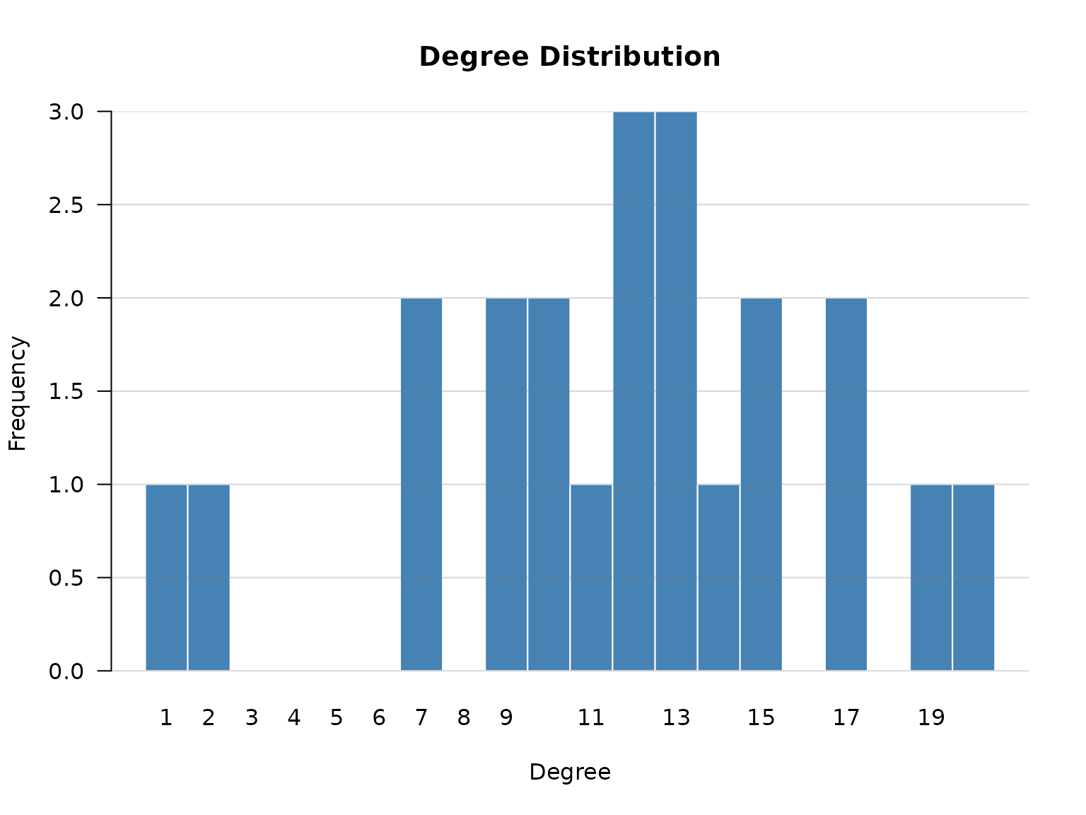
Comparing similarity measures
Each similarity measure surfaces different structure in the data, prioritizing different aspects of co-occurrence. The examples below show the top 3 pairs under each measure using a movie genres dataset.
-
similarity = "none"— Raw counts favor the most frequent genre pairs. Drama dominates because it is the most common genre, so its co-occurrences with Comedy and Romance rank highest regardless of how strongly the genres are actually associated.
co(movies, field = "genres", sep = ",", similarity = "none", top_n = 3)
#> # cooccurrence: 22 nodes, 3 edges | density: 0.0130 | mean degree: 0.2727 | 1000 transactions
#> # similarity: none | counting: full
#> # possible edges: 231 | isolates: 18
#> # top nodes: Drama(deg=3,str=381), Comedy(deg=1,str=159), Romance(deg=1,str=131), Crime(deg=1,str=91)
#>    from      to weight count
#>  Comedy   Drama    159   159
#>   Drama Romance    131   131
#> Crime Drama 91 91-
similarity = "jaccard"— Normalizing by the union of occurrences brings less frequent but more tightly associated pairs to the top. Adventure–Animation emerges as the strongest pair, suggesting these genres appear together more consistently relative to how often either appears alone.
co(movies, field = "genres", sep = ",", similarity = "jaccard", top_n = 3)
#> # cooccurrence: 22 nodes, 3 edges | density: 0.0130 | mean degree: 0.2727 | 1000 transactions
#> # similarity: jaccard | counting: full
#> # possible edges: 231 | isolates: 16
#> # top nodes: Adventure(deg=1,str=0.2847), Animation(deg=1,str=0.2847), Action(deg=1,str=0.2369), Crime(deg=1,str=0.2369), Comedy(deg=1,str=0.2112)
#>       from        to    weight count
#>  Adventure Animation 0.2846715    39
#>     Action     Crime 0.2369478    59
#> Comedy Drama 0.2111554 159-
similarity = "cosine"— Similar to Jaccard but less strict, cosine also elevates Adventure–Animation while keeping Drama–Romance in the top 3, reflecting its more lenient treatment of frequency differences between genres.
co(movies, field = "genres", sep = ",", similarity = "cosine", top_n = 3)
#> # cooccurrence: 22 nodes, 3 edges | density: 0.0130 | mean degree: 0.2727 | 1000 transactions
#> # similarity: cosine | counting: full
#> # possible edges: 231 | isolates: 16
#> # top nodes: Adventure(deg=1,str=0.4481), Animation(deg=1,str=0.4481), Drama(deg=1,str=0.4113), Romance(deg=1,str=0.4113), Action(deg=1,str=0.3831)
#>       from        to    weight count
#>  Adventure Animation 0.4480983    39
#>      Drama   Romance 0.4113075   131
#> Action Crime 0.3831250 59-
similarity = "inclusion"— Dividing by the less common genre’s frequency surfaces subset relationships. Documentary–News and History–News both score 1, meaning News movies are always also tagged as Documentary or History—News is a niche genre that only appears alongside broader ones.
co(movies, field = "genres", sep = ",", similarity = "inclusion", top_n = 3)
#> # cooccurrence: 22 nodes, 3 edges | density: 0.0130 | mean degree: 0.2727 | 1000 transactions
#> # similarity: inclusion | counting: full
#> # possible edges: 231 | isolates: 17
#> # top nodes: News(deg=2,str=2), Documentary(deg=1,str=1), Drama(deg=1,str=1), History(deg=1,str=1), Western(deg=1,str=1)
#>         from      to weight count
#>  Documentary    News      1     1
#>      History    News      1     1
#> Drama Western 1 1-
similarity = "association"— Discounting by the product of individual frequencies reveals pairs that co-occur far more than chance would predict. Rare genre combinations like History–News and Documentary–News top the list because their co-occurrence is disproportionately high relative to their individual frequencies.
co(movies, field = "genres", sep = ",", similarity = "association", top_n = 3)
#> # cooccurrence: 22 nodes, 3 edges | density: 0.0130 | mean degree: 0.2727 | 1000 transactions
#> # similarity: association | counting: full
#> # possible edges: 231 | isolates: 17
#> # top nodes: News(deg=2,str=0.02271), History(deg=1,str=0.01613), Horror(deg=1,str=0.01136), Sci-Fi(deg=1,str=0.01136), Documentary(deg=1,str=0.006579)
#>         from     to      weight count
#>      History   News 0.016129032     1
#>       Horror Sci-Fi 0.011363636     2
#> Documentary News 0.006578947 1-
similarity = "dice"— Results closely mirror Jaccard, with the same top pairs appearing in the same order but with slightly higher weights — reflecting Dice’s more lenient arithmetic mean normalization. Adventure-Animation, Action-Crime, and Comedy-Drama remain the strongest genre affinities, with Comedy-Drama recording the highest raw co-occurrence count at 159 despite its comparatively lower weight, indicating that both genres are individually common but not exclusively paired.
co(movies, field = "genres", sep = ",", similarity = "dice", top_n = 3)
#> # cooccurrence: 22 nodes, 3 edges | density: 0.0130 | mean degree: 0.2727 | 1000 transactions
#> # similarity: dice | counting: full
#> # possible edges: 231 | isolates: 16
#> # top nodes: Adventure(deg=1,str=0.4432), Animation(deg=1,str=0.4432), Action(deg=1,str=0.3831), Crime(deg=1,str=0.3831), Comedy(deg=1,str=0.3487)
#>       from        to    weight count
#>  Adventure Animation 0.4431818    39
#>     Action     Crime 0.3831169    59
#> Comedy Drama 0.3486842 159-
similarity = "equivalence"— Squaring the cosine amplifies differences between strong and weak pairs, pushing weaker associations further down the rankings. Adventure-Animation retains the top spot, but Drama–Romance displaces Action-Crime into third place, suggesting that while Action-Crime has a higher raw count, Drama–Romance represents a tighter and more exclusive pairing once the penalty for common genres is compounded.
co(movies, field = "genres", sep = ",", similarity = "equivalence", top_n = 3)
#> # cooccurrence: 22 nodes, 3 edges | density: 0.0130 | mean degree: 0.2727 | 1000 transactions
#> # similarity: equivalence | counting: full
#> # possible edges: 231 | isolates: 16
#> # top nodes: Adventure(deg=1,str=0.2008), Animation(deg=1,str=0.2008), Drama(deg=1,str=0.1692), Romance(deg=1,str=0.1692), Action(deg=1,str=0.1468)
#>       from        to    weight count
#>  Adventure Animation 0.2007921    39
#>      Drama   Romance 0.1691739   131
#>     Action     Crime 0.1467847    59
Which similarity to use?
-
Exploratory work: Start with
"none"to see raw counts and understand the data, then try"jaccard"or"cosine"for a balanced view. -
Bibliometric and scientometric networks:
"association"is recommended by van Eck & Waltman (2009) because it correctly accounts for the expected number of co-occurrences under independence. Two items that are both very frequent will naturally co-occur often; association strength discounts this, revealing which pairs co-occur more than chance alone would predict. -
Detecting hierarchical or subset structure:
"inclusion"(the Simpson coefficient) reveals when one item almost always appears with another — useful for identifying items that are subsets of broader categories, or for detecting dependency relationships. -
Binary presence/absence networks:
"jaccard"or"dice"when you only care whether items co-occur, not how often. Jaccard is stricter (penalizes unbalanced pairs more); Dice is more lenient. -
Scale-invariant comparison:
"cosine"is invariant to absolute frequency — useful when comparing co-occurrence patterns across datasets of different sizes. -
Strict filtering:
"equivalence"(cosine squared) amplifies differences — pairs with weak overlap get pushed closer to zero, retaining only the strongest associations.
2. Counting methods
By default, each transaction contributes equally to co-occurrence counts: if a movie has genres A, B, and C, each pair adds 1. This means movies with many genres inflate the network — a 5-genre movie creates 10 pairs, while a 2-genre movie creates only 1, giving multi-genre movies disproportionate influence.
Fractional counting addresses this by weighting each pair by , where is the number of items in the transaction, so every transaction contributes equally regardless of how many genres it contains.
co(movies, field = "genres", sep = ",", top_n = 5)
#> # cooccurrence: 22 nodes, 5 edges | density: 0.0216 | mean degree: 0.4545 | 1000 transactions
#> # similarity: none | counting: full
#> # possible edges: 231 | isolates: 17
#> # top nodes: Drama(deg=4,str=452), Comedy(deg=2,str=222), Romance(deg=2,str=194), Crime(deg=1,str=91), Action(deg=1,str=71)
#>    from      to weight count
#>  Comedy   Drama    159   159
#>   Drama Romance    131   131
#>   Crime   Drama     91    91
#>  Action   Drama     71    71
#>  Comedy Romance     63    63
co(movies, field = "genres", sep = ",", counting = "fractional", top_n = 5)
#> # cooccurrence: 22 nodes, 5 edges | density: 0.0216 | mean degree: 0.4545 | 1000 transactions
#> # similarity: none | counting: fractional
#> # possible edges: 231 | isolates: 17
#> # top nodes: Drama(deg=4,str=293), Comedy(deg=2,str=146), Romance(deg=2,str=133), Crime(deg=1,str=52.5), Action(deg=1,str=38.5)
#>    from      to weight count
#>  Comedy   Drama  107.5   159
#>   Drama Romance   94.5   131
#>   Crime   Drama   52.5    91
#>  Action   Drama   38.5    71
#>  Comedy Romance   38.5    63
The top pairs remain the same under both methods, but the weights are lower under fractional counting. For example, Comedy-Drama drops from 159 to 107.5, reflecting the downweighting of multi-genre movies that contributed to this pair. Fractional counting is particularly important when some transactions contain many items while others contain few, as it prevents high-cardinality transactions from dominating the network.
3. Scaling
Scaling compresses or transforms the weight distribution after similarity normalization, making it easier to visualize or use in downstream analysis. Scaling can be applied on its own or combined with any similarity measure.
-
scale = "log"— Applies a natural log transformation, compressing the heavy tail of the distribution. The ranking of pairs is preserved but the gap between frequent and infrequent pairs is reduced. Comedy-Drama and Drama-Romance* remain at the top, but their weights are now much closer together than raw counts would suggest.
co(movies, field = "genres", sep = ",", scale = "log", top_n = 5)
#> # cooccurrence: 22 nodes, 5 edges | density: 0.0216 | mean degree: 0.4545 | 1000 transactions
#> # similarity: none | counting: full | scale: log
#> # possible edges: 231 | isolates: 17
#> # top nodes: Drama(deg=4,str=18.76), Comedy(deg=2,str=9.234), Romance(deg=2,str=9.042), Crime(deg=1,str=4.522), Action(deg=1,str=4.277)
#>    from      to   weight count
#>  Comedy   Drama 5.075174   159
#>   Drama Romance 4.882802   131
#>   Crime   Drama 4.521789    91
#>  Action   Drama 4.276666    71
#> Comedy Romance 4.158883 63-
scale = "minmax"— Rescales all weights to the range [0, 1], where the strongest pair scores 1 and all others are expressed relative to it. Useful for comparing networks of different sizes or when absolute counts are not meaningful. Adventure-Animation scores a perfect 1 as the strongest Jaccard pair in the network. Biography-Documentary reaches the top 5 with a raw count of only 44, indicating that when these genres appear together they do so with high exclusivity relative to how often either appears alone.
co(movies, field = "genres", sep = ",", similarity = "jaccard", scale = "minmax", top_n = 5)
#> # cooccurrence: 22 nodes, 5 edges | density: 0.0216 | mean degree: 0.4545 | 1000 transactions
#> # similarity: jaccard | counting: full | scale: minmax
#> # possible edges: 231 | isolates: 14
#> # top nodes: Adventure(deg=2,str=1.728), Action(deg=2,str=1.559), Animation(deg=1,str=1), Crime(deg=1,str=0.8314), Comedy(deg=1,str=0.7403)
#>       from          to    weight count
#>  Adventure   Animation 1.0000000    39
#>     Action       Crime 0.8314210    59
#>     Comedy       Drama 0.7403121   159
#>     Action   Adventure 0.7275665    44
#> Biography Documentary 0.7139898 44-
scale = "binary"— Converts all positive weights to 1, producing a presence/absence network. The top pairs are no longer ranked by strength but simply by whether they co-occur at all. Action-Adventure dominate simply because they appear together across a wide range of combinations.
co(movies, field = "genres", sep = ",", scale = "binary", top_n = 5)
#> # cooccurrence: 22 nodes, 5 edges | density: 0.0216 | mean degree: 0.4545 | 1000 transactions
#> # similarity: none | counting: full | scale: binary
#> # possible edges: 231 | isolates: 18
#> # top nodes: Action(deg=3,str=3), Adventure(deg=3,str=3), Animation(deg=2,str=2), Biography(deg=2,str=2)
#>       from        to weight count
#>     Action Adventure      1    44
#>     Action Animation      1    27
#>  Adventure Animation      1    39
#>     Action Biography      1     5
#> Adventure Biography 1 8-
scale = "sqrt"— Applies a square root transformation, providing a milder compression than log. The ranking is preserved and the distribution is slightly less skewed than the raw counts. Comedy-Drama leads with a weight of 12.6 compared to Comedy-Romance at 7.9, a smaller proportional gap than the raw count difference of 159 versus 63 would imply.
co(movies, field = "genres", sep = ",", scale = "sqrt", top_n = 5)
#> # cooccurrence: 22 nodes, 5 edges | density: 0.0216 | mean degree: 0.4545 | 1000 transactions
#> # similarity: none | counting: full | scale: sqrt
#> # possible edges: 231 | isolates: 17
#> # top nodes: Drama(deg=4,str=42.02), Comedy(deg=2,str=20.55), Romance(deg=2,str=19.38), Crime(deg=1,str=9.539), Action(deg=1,str=8.426)
#>    from      to    weight count
#>  Comedy   Drama 12.609520   159
#>   Drama Romance 11.445523   131
#>   Crime   Drama  9.539392    91
#>  Action   Drama  8.426150    71
#>  Comedy Romance  7.937254    63
Scaling can be combined with any similarity measure and with filtering arguments. The example below applies association strength followed by log scaling, retaining only genres appearing in at least 20 movies. Drama-heavy pairs drop out entirely once popularity is penalized, and niche but tightly linked pairs like Adventure-Animation, History-War, and Mystery-Thriller rise to the top, reflecting genres that genuinely cluster together rather than simply co-occurring by volume.
co(movies, field = "genres", sep = ",",
   similarity = "association", scale = "log", min_occur = 20, top_n = 5)
#> # cooccurrence: 17 nodes, 5 edges | density: 0.0368 | mean degree: 0.5882 | 998 transactions
#> # similarity: association | counting: full | scale: log
#> # possible edges: 136 | isolates: 8
#> # top nodes: Animation(deg=2,str=0.008659), Adventure(deg=1,str=0.005135), History(deg=1,str=0.004526), War(deg=1,str=0.004526), Mystery(deg=1,str=0.003804)
#>         from        to      weight count
#>    Adventure Animation 0.005135307    39
#>      History       War 0.004526032     9
#>      Mystery  Thriller 0.003803732    15
#>  Documentary     Music 0.003536250    28
#>    Animation   Fantasy 0.003523198     9
4. Filtering
Three filtering arguments control which edges appear in the result. They can be used independently or combined.
-
min_occur— Drops any genre appearing in fewer than the specified number of transactions before co-occurrences are computed, removing rare items that would otherwise inflate the edge count. Here only movies with co-occurrence of minimum 20 are kept.
co(movies, field = "genres", sep = ",", similarity = "jaccard", min_occur = 20)
#> # cooccurrence: 17 nodes, 102 edges | density: 0.7500 | mean degree: 12.0000 | 998 transactions
#> # similarity: jaccard | counting: full
#> # possible edges: 136 | isolates: 0
#> # top nodes: Drama(deg=16,str=1.153), Comedy(deg=16,str=0.8949), Romance(deg=15,str=0.5377), Action(deg=14,str=1.009), Adventure(deg=14,str=0.8788)
#>         from          to    weight count
#>    Adventure   Animation 0.2846715    39
#>       Action       Crime 0.2369478    59
#>       Comedy       Drama 0.2111554   159
#>       Action   Adventure 0.2075472    44
#>    Biography Documentary 0.2037037    44
#>        Drama     Romance 0.1975867   131
#>        Crime    Thriller 0.1745283    37
#>       Comedy     Romance 0.1680000    63
#>  Documentary       Music 0.1590909    28
#>    Biography     History 0.1564626    23
#> # ... 92 more edges-
threshold— Retains only edges with a weight at or above the specified value, applied after similarity normalization and scaling. Here only pairs with a Jaccard similarity above 0.15 are kept.
co(movies, field = "genres", sep = ",", similarity = "jaccard", threshold = 0.15)
#> # cooccurrence: 22 nodes, 10 edges | density: 0.0433 | mean degree: 0.9091 | 1000 transactions
#> # similarity: jaccard | counting: full
#> # possible edges: 231 | isolates: 10
#> # top nodes: Adventure(deg=2,str=0.4922), Action(deg=2,str=0.4445), Crime(deg=2,str=0.4115), Drama(deg=2,str=0.4087), Comedy(deg=2,str=0.3792)
#>         from          to    weight count
#>    Adventure   Animation 0.2846715    39
#>       Action       Crime 0.2369478    59
#>       Comedy       Drama 0.2111554   159
#>       Action   Adventure 0.2075472    44
#>    Biography Documentary 0.2037037    44
#>        Drama     Romance 0.1975867   131
#>        Crime    Thriller 0.1745283    37
#>       Comedy     Romance 0.1680000    63
#>  Documentary       Music 0.1590909    28
#> Biography History 0.1564626 23-
top_n— Keeps only the n strongest edges by weight, regardless of their absolute value.
co(movies, field = "genres", sep = ",", similarity = "jaccard", top_n = 10)
#> # cooccurrence: 22 nodes, 10 edges | density: 0.0433 | mean degree: 0.9091 | 1000 transactions
#> # similarity: jaccard | counting: full
#> # possible edges: 231 | isolates: 10
#> # top nodes: Adventure(deg=2,str=0.4922), Action(deg=2,str=0.4445), Crime(deg=2,str=0.4115), Drama(deg=2,str=0.4087), Comedy(deg=2,str=0.3792)
#>         from          to    weight count
#>    Adventure   Animation 0.2846715    39
#>       Action       Crime 0.2369478    59
#>       Comedy       Drama 0.2111554   159
#>       Action   Adventure 0.2075472    44
#>    Biography Documentary 0.2037037    44
#>        Drama     Romance 0.1975867   131
#>        Crime    Thriller 0.1745283    37
#>       Comedy     Romance 0.1680000    63
#>  Documentary       Music 0.1590909    28
#>    Biography     History 0.1564626    23
All three thresholds can be combined for fine-grained control over network size and density:
co(movies, field = "genres", sep = ",",
   similarity = "association", counting = "fractional",
   min_occur = 15, threshold = 0.001, top_n = 20)
#> # cooccurrence: 18 nodes, 20 edges | density: 0.1307 | mean degree: 2.2222 | 999 transactions
#> # similarity: association | counting: fractional
#> # possible edges: 153 | isolates: 3
#> # top nodes: Animation(deg=4,str=0.007167), Adventure(deg=4,str=0.006691), Action(deg=4,str=0.005445), Documentary(deg=3,str=0.006946), Thriller(deg=3,str=0.004857)
#>         from          to      weight count
#>  Documentary       Music 0.002973178    28
#>    Adventure   Animation 0.002574257    39
#>      History         War 0.002268145     9
#>      Mystery    Thriller 0.002159553    15
#>  Documentary       Sport 0.002114662    11
#>    Biography Documentary 0.001857943    44
#>    Animation     Fantasy 0.001764706     9
#>    Biography     History 0.001717443    23
#>    Animation      Family 0.001666667     9
#>       Family     Fantasy 0.001633987     4
#> # ... 10 more edges
5. Actor co-occurrence (long/bipartite format)
Actors who appear in the same movie are connected. The data has one
row per actor–movie pair, making it a natural fit for the long/bipartite
format. The field argument specifies the entity column and
by specifies the grouping column.
co(actors, field = "actor", by = "tconst",
   similarity = "jaccard", min_occur = 3, threshold = 0.1)
#> # cooccurrence: 19 nodes, 7 edges | density: 0.0409 | mean degree: 0.7368 | 47 transactions
#> # similarity: jaccard | counting: full
#> # possible edges: 171 | isolates: 7
#> # top nodes: Dina Pathak(deg=2,str=0.4), Mukesh(deg=2,str=0.4), Julia Bache-Wiig(deg=1,str=1), Robin Ottersen(deg=1,str=1), Constantin Fleancu(deg=1,str=0.5)
#>                from             to weight count
#>    Julia Bache-Wiig Robin Ottersen    1.0     3
#>  Constantin Fleancu Liliana Mocanu    0.5     2
#>         Dina Pathak   Harish Magon    0.2     1
#>         Dina Pathak         Mukesh    0.2     1
#>           Akash Dev         Rajesh    0.2     1
#>         Joseph Izzo    Shiyoon Kim    0.2     1
#>              Mukesh          Vinod    0.2     1
Julia Bache-Wiig and Robin Ottersen score 1.0, meaning they appear together in every movie either of them appears in — a perfect Jaccard score. Applying fractional counting downweights pairs from movies with large casts, though in this case the results are unchanged because the dataset is small and cast sizes are similar across movies.
co(actors, field = "actor", by = "tconst",
   similarity = "jaccard", counting = "fractional",
   min_occur = 3, threshold = 0.05)
#> # cooccurrence: 19 nodes, 7 edges | density: 0.0409 | mean degree: 0.7368 | 47 transactions
#> # similarity: jaccard | counting: fractional
#> # possible edges: 171 | isolates: 7
#> # top nodes: Dina Pathak(deg=2,str=0.4), Mukesh(deg=2,str=0.4), Julia Bache-Wiig(deg=1,str=1), Robin Ottersen(deg=1,str=1), Constantin Fleancu(deg=1,str=0.5)
#>                from             to weight count
#>    Julia Bache-Wiig Robin Ottersen    1.0     3
#>  Constantin Fleancu Liliana Mocanu    0.5     2
#>         Dina Pathak   Harish Magon    0.2     1
#>         Dina Pathak         Mukesh    0.2     1
#>           Akash Dev         Rajesh    0.2     1
#>         Joseph Izzo    Shiyoon Kim    0.2     1
#>              Mukesh          Vinod    0.2     1
6. Splitting by groups
The split_by argument computes a separate co-occurrence network for each level of a grouping variable and returns all results in a single data frame with a group column.
-
split_by = "decade"— Each decade gets its own Jaccard-weighted genre network. The dominant pairs shift across decades, reflecting how genre combinations have changed over time.
co(movies, field = "genres", sep = ",",
   split_by = "decade", similarity = "jaccard",
   min_occur = 5, top_n = 5)
#> # cooccurrence: 15 nodes, 30 edges
#> # split_by: decade (6 groups)
#> # similarity: jaccard | counting: full
#> # isolates: 0 | per-group metrics: summary()
#>         from        to    weight count group
#>    Adventure Animation 0.5000000     7 1970s
#>        Crime  Thriller 0.4285714     6 1970s
#>    Biography   History 0.3333333     4 1970s
#>    Animation    Family 0.2500000     3 1970s
#>    Animation    Comedy 0.2258065     7 1970s
#>  Documentary     Music 0.4444444     4 1980s
#>       Action     Crime 0.2333333     7 1980s
#>    Biography   History 0.2142857     3 1980s
#>       Comedy     Drama 0.2043011    19 1980s
#>        Crime     Drama 0.2027027    15 1980s
#> # ... 20 more edges
Individual groups can be extracted with subset() on the
group column:
decades <- co(movies, field = "genres", sep = ",",
              split_by = "decade", similarity = "jaccard",
              min_occur = 5, top_n = 5)

subset(decades, group == "2010s")
#> # cooccurrence: 8 nodes, 5 edges
#> # similarity: none | counting: full
#> # isolates: 0 | per-group metrics: summary()
#>       from          to    weight count group
#>     Action       Crime 0.2988506    26 2010s
#>  Adventure   Animation 0.2884615    15 2010s
#>  Biography Documentary 0.2872340    27 2010s
#>     Action   Adventure 0.1951220    16 2010s
#>     Comedy       Drama 0.1911111    43 2010s
Group-level network metrics come from summary() as a
tidy data frame:
decade_summary <- summary(decades)
#> cooccurrence network
#> ------------------------------
#> Nodes          : 15
#> Edges          : 30 (pooled across groups)
#> Isolates       : 0
#> Split by       : decade (6 groups)
#> Similarity     : jaccard
#> Counting       : full
#> Weight range   : [0.1889, 0.5]
#> Weight mean    : 0.2731
#> Count range    : [3, 43]
#> Count mean     : 13.73
#> Groups         : 1970s(12 nodes, 5 edges, 0.0758 density), 1980s(14 nodes, 5 edges, 0.0549 density), 1990s(13 nodes, 5 edges, 0.0641 density), 2000s(16 nodes, 5 edges, 0.0417 density), 2010s(17 nodes, 5 edges, 0.0368 density)

as.data.frame(decade_summary, what = "groups")
#>   group n_nodes n_edges possible_edges    density weight_mean count_sum
#> 1 1970s      12       5             66 0.07575758   0.3475422        27
#> 2 1980s      14       5             91 0.05494505   0.2598135        48
#> 3 1990s      13       5             78 0.06410256   0.2959117        69
#> 4 2000s      16       5            120 0.04166667   0.2316965        99
#> 5 2010s      17       5            136 0.03676471   0.2521558       127
#> 6 2020s 13 5 78 0.06410256 0.2512590 42-
split_by = "rating_band"— Splitting by rating band reveals whether highly rated movies have different genre co-occurrence patterns than average-rated ones. Documentary–Music is the strongest pair among top-rated movies, while Adventure–Animation leads among the 7–7.9 band.
movies$rating_band <- ifelse(movies$averageRating >= 8, "8+", "7-7.9")
co(movies, field = "genres", sep = ",",
   split_by = "rating_band", similarity = "jaccard",
   min_occur = 10, top_n = 5)
#> # cooccurrence: 10 nodes, 10 edges
#> # split_by: rating_band (2 groups)
#> # similarity: jaccard | counting: full
#> # isolates: 0 | per-group metrics: summary()
#>         from          to    weight count group
#>    Adventure   Animation 0.2926829    36 7-7.9
#>       Action       Crime 0.2477477    55 7-7.9
#>       Comedy       Drama 0.2130898   140 7-7.9
#>       Action   Adventure 0.2116402    40 7-7.9
#>    Biography Documentary 0.2111111    38 7-7.9
#>  Documentary       Music 0.3333333    10    8+
#>       Comedy       Drama 0.1979167    19    8+
#>    Biography Documentary 0.1666667     6    8+
#>       Comedy     Romance 0.1555556     7    8+
#>        Drama     Romance 0.1547619    13    8+
7. Output formats
The default output format returns a tidy data frame with
from, to, weight, and
count columns, ready for further analysis or
visualization.
co(movies, field = "genres", sep = ",", top_n = 5)
#> # cooccurrence: 22 nodes, 5 edges | density: 0.0216 | mean degree: 0.4545 | 1000 transactions
#> # similarity: none | counting: full
#> # possible edges: 231 | isolates: 17
#> # top nodes: Drama(deg=4,str=452), Comedy(deg=2,str=222), Romance(deg=2,str=194), Crime(deg=1,str=91), Action(deg=1,str=71)
#>    from      to weight count
#>  Comedy   Drama    159   159
#>   Drama Romance    131   131
#>   Crime   Drama     91    91
#>  Action   Drama     71    71
#>  Comedy Romance     63    63
Gephi
The Gephi output format returns a data frame formatted for direct
import into Gephi, with Source, Target,
Weight, Type, and Count columns.
The result can be written straight to CSV.
co(movies, field = "genres", sep = ",",
   similarity = "jaccard", output = "gephi", top_n = 10)
#> # cooccurrence: 22 nodes, 10 edges | density: 0.0433 | mean degree: 0.9091 | 1000 transactions
#> # similarity: jaccard | counting: full
#> # possible edges: 231 | isolates: 10
#> # top nodes: Adventure(deg=2,str=0.4922), Action(deg=2,str=0.4445), Crime(deg=2,str=0.4115), Drama(deg=2,str=0.4087), Comedy(deg=2,str=0.3792)
#>       Source      Target    Weight       Type Count
#>    Adventure   Animation 0.2846715 Undirected    39
#>       Action       Crime 0.2369478 Undirected    59
#>       Comedy       Drama 0.2111554 Undirected   159
#>       Action   Adventure 0.2075472 Undirected    44
#>    Biography Documentary 0.2037037 Undirected    44
#>        Drama     Romance 0.1975867 Undirected   131
#>        Crime    Thriller 0.1745283 Undirected    37
#>       Comedy     Romance 0.1680000 Undirected    63
#>  Documentary       Music 0.1590909 Undirected    28
#> Biography History 0.1564626 Undirected 23cograph (with Gephi layout)
The cograph output format returns a cograph_network
object that can be passed directly to splot() for
visualization. The layout argument controls the node placement algorithm
— "fr" uses Fruchterman-Reingold, and
scale_nodes_by = "degree" sizes nodes by their degree
centrality.
library(cograph)
net <- co(movies, field = "genres", sep = ",",
          similarity = "jaccard", min_occur = 20, output = "cograph")
splot(net, layout = "fr", scale_nodes_by = "degree")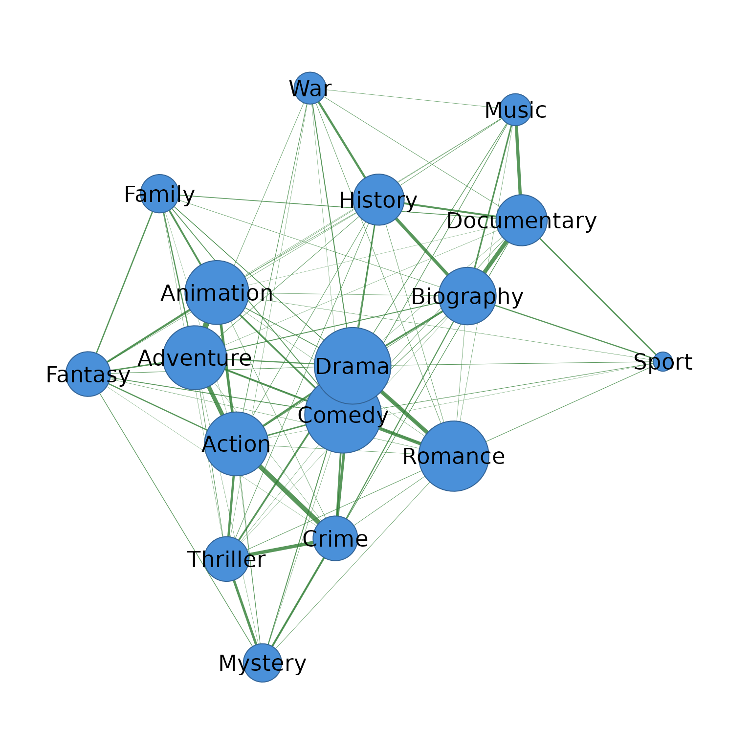
Additional styling arguments control edge_width_range,
label_size, node_color, and
node_border_width:
library(cograph)
splot(net, layout = "gephi", label_size = .8, label_fontface = "bold",
           node_fill = "#F9C22E",
           node_border_width = 0.0001, edge_color = "black",
           scale_nodes_by = "degree", edge_width_range = c(0.1:4))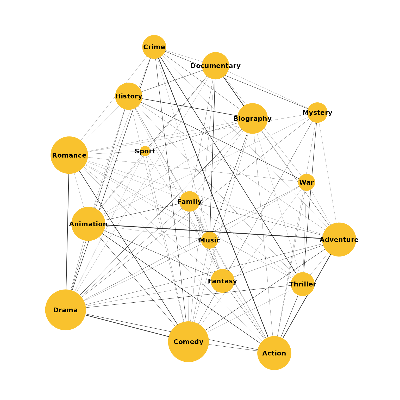
igraph
The igraph output format returns an igraph object. All
standard igraph functions work on the result without any conversion.
g <- co(movies, field = "genres", sep = ",",
        similarity = "jaccard", min_occur = 20, output = "igraph")
g
#> IGRAPH 9248606 UNW- 17 102 --
#> + attr: name (v/c), weight (e/n), count (e/n)
#> + edges from 9248606 (vertex names):
#>  [1] Adventure  --Animation   Action     --Crime       Comedy     --Drama
#>  [4] Action     --Adventure   Biography  --Documentary Drama      --Romance
#>  [7] Crime      --Thriller    Comedy     --Romance     Documentary--Music
#> [10] Biography  --History     Action     --Animation   Crime      --Drama
#> [13] Mystery    --Thriller    Action     --Thriller    History    --War
#> [16] Action     --Drama       Crime      --Mystery     Documentary--History
#> [19] Animation  --Fantasy     Adventure  --Comedy      Animation  --Family
#> [22] Biography  --Drama       Drama      --Thriller    Comedy     --Crime
#> + ... omitted several edges
Centrality measures can be computed directly on the
igraph object:
igraph::degree(g)
#>      Action   Adventure   Animation   Biography      Comedy       Crime
#>          14          14          14          13          16          11
#> Documentary       Drama      Family     Fantasy     History       Music
#>          12          16          10          11          12           9
#>     Mystery     Romance       Sport    Thriller         War
#>          10          15           7          11           9
igraph::betweenness(g)
#>      Action   Adventure   Animation   Biography      Comedy       Crime
#>           6           7          25           3           3           4
#> Documentary       Drama      Family     Fantasy     History       Music
#>          15           0          17           6           1           2
#>     Mystery     Romance       Sport    Thriller         War
#>           3          18           3          11           2
Matrix
The matrix output format returns a square co-occurrence matrix where rows and columns are items and each cell contains the similarity weight between the corresponding pair. This is useful for downstream analysis that expects a matrix input, such as clustering or heatmap visualization.
mat <- co(movies, field = "genres", sep = ",",
          similarity = "jaccard", min_occur = 20, output = "matrix")
round(mat[1:6, 1:6], 3)
#>           Action Adventure Animation Biography Comedy Crime
#> Action     0.000     0.208     0.133     0.019  0.067 0.237
#> Adventure  0.208     0.000     0.285     0.040  0.089 0.008
#> Animation  0.133     0.285     0.000     0.011  0.083 0.013
#> Biography  0.019     0.040     0.011     0.000  0.021 0.048
#> Comedy     0.067     0.089     0.083     0.021  0.000 0.083
#> Crime      0.237     0.008     0.013     0.048  0.083 0.000
8. Converters
Converters transform a cooccurrence result into other
formats after the fact, without re-running the computation. This is
useful when you want to start with the default tidy data frame and
convert to a specific format only when needed.
as_matrix() converts the result to a square similarity
matrix, where each cell contains the Jaccard weight between the
corresponding pair of genres:
result <- co(movies, field = "genres", sep = ",",
             similarity = "jaccard", min_occur = 20)
as_matrix(result)
#>                  Action   Adventure   Animation   Biography      Comedy
#> Action      0.000000000 0.207547170 0.133004926 0.019379845 0.066502463
#> Adventure   0.207547170 0.000000000 0.284671533 0.039800995 0.089080460
#> Animation   0.133004926 0.284671533 0.000000000 0.011049724 0.082822086
#> Biography   0.019379845 0.039800995 0.011049724 0.000000000 0.021164021
#> Comedy      0.066502463 0.089080460 0.082822086 0.021164021 0.000000000
#> Crime       0.236947791 0.007936508 0.013333333 0.048192771 0.082914573
#> Documentary 0.000000000 0.007968127 0.004424779 0.203703704 0.016548463
#> Drama       0.098885794 0.051502146 0.033527697 0.086383602 0.211155378
#> Family      0.005263158 0.053846154 0.088235294 0.014084507 0.036303630
#> Fantasy     0.055865922 0.062992126 0.090000000 0.000000000 0.036544850
#> History     0.018779343 0.018750000 0.014814815 0.156462585 0.014925373
#> Music       0.000000000 0.000000000 0.007936508 0.073825503 0.024844720
#> Mystery     0.015544041 0.007092199 0.008695652 0.000000000 0.009493671
#> Romance     0.012861736 0.011627907 0.008583691 0.011320755 0.168000000
#> Sport       0.005494505 0.000000000 0.009803922 0.054263566 0.020000000
#> Thriller    0.110619469 0.020725389 0.000000000 0.004926108 0.008086253
#> War         0.021857923 0.015267176 0.000000000 0.000000000 0.006493506
#>                   Crime Documentary       Drama      Family     Fantasy
#> Action      0.236947791 0.000000000 0.098885794 0.005263158 0.055865922
#> Adventure   0.007936508 0.007968127 0.051502146 0.053846154 0.062992126
#> Animation   0.013333333 0.004424779 0.033527697 0.088235294 0.090000000
#> Biography   0.048192771 0.203703704 0.086383602 0.014084507 0.000000000
#> Comedy      0.082914573 0.016548463 0.211155378 0.036303630 0.036544850
#> Crime       0.000000000 0.016666667 0.130747126 0.000000000 0.005376344
#> Documentary 0.016666667 0.000000000 0.007692308 0.032967033 0.000000000
#> Drama       0.130747126 0.007692308 0.000000000 0.030769231 0.021406728
#> Family      0.000000000 0.032967033 0.030769231 0.000000000 0.060606061
#> Fantasy     0.005376344 0.000000000 0.021406728 0.060606061 0.000000000
#> History     0.000000000 0.091836735 0.065849923 0.000000000 0.010526316
#> Music       0.000000000 0.159090909 0.026946108 0.000000000 0.011764706
#> Mystery     0.096045198 0.010471204 0.041666667 0.000000000 0.027397260
#> Romance     0.016233766 0.000000000 0.197586727 0.005128205 0.010416667
#> Sport       0.000000000 0.065088757 0.021604938 0.000000000 0.000000000
#> Thriller    0.174528302 0.000000000 0.084695394 0.007633588 0.000000000
#> War         0.000000000 0.016574586 0.042253521 0.000000000 0.000000000
#>                History       Music     Mystery     Romance       Sport
#> Action      0.01877934 0.000000000 0.015544041 0.012861736 0.005494505
#> Adventure   0.01875000 0.000000000 0.007092199 0.011627907 0.000000000
#> Animation   0.01481481 0.007936508 0.008695652 0.008583691 0.009803922
#> Biography   0.15646259 0.073825503 0.000000000 0.011320755 0.054263566
#> Comedy      0.01492537 0.024844720 0.009493671 0.168000000 0.020000000
#> Crime       0.00000000 0.000000000 0.096045198 0.016233766 0.000000000
#> Documentary 0.09183673 0.159090909 0.010471204 0.000000000 0.065088757
#> Drama       0.06584992 0.026946108 0.041666667 0.197586727 0.021604938
#> Family      0.00000000 0.000000000 0.000000000 0.005128205 0.000000000
#> Fantasy     0.01052632 0.011764706 0.027397260 0.010416667 0.000000000
#> History     0.00000000 0.017857143 0.000000000 0.013698630 0.000000000
#> Music       0.01785714 0.000000000 0.000000000 0.009523810 0.000000000
#> Mystery     0.00000000 0.000000000 0.000000000 0.015151515 0.000000000
#> Romance     0.01369863 0.009523810 0.015151515 0.000000000 0.021739130
#> Sport       0.00000000 0.000000000 0.000000000 0.021739130 0.000000000
#> Thriller    0.01935484 0.000000000 0.122950820 0.019920319 0.000000000
#> War         0.10588235 0.012048193 0.000000000 0.015873016 0.000000000
#>                Thriller         War
#> Action      0.110619469 0.021857923
#> Adventure   0.020725389 0.015267176
#> Animation   0.000000000 0.000000000
#> Biography   0.004926108 0.000000000
#> Comedy      0.008086253 0.006493506
#> Crime       0.174528302 0.000000000
#> Documentary 0.000000000 0.016574586
#> Drama       0.084695394 0.042253521
#> Family      0.007633588 0.000000000
#> Fantasy     0.000000000 0.000000000
#> History     0.019354839 0.105882353
#> Music       0.000000000 0.012048193
#> Mystery     0.122950820 0.000000000
#> Romance     0.019920319 0.015873016
#> Sport       0.000000000 0.000000000
#> Thriller    0.000000000 0.007874016
#> War         0.007874016 0.000000000
as_matrix(result, type = "raw") returns the raw
co-occurrence count matrix instead, with no similarity normalization
applied:
as_matrix(result, type = "raw")
#>             Action Adventure Animation Biography Comedy Crime Documentary Drama
#> Action           0        44        27         5     27    59           0    71
#> Adventure       44         0        39         8     31     2           2    36
#> Animation       27        39         0         2     27     3           1    23
#> Biography        5         8         2         0      8    12          44    59
#> Comedy          27        31        27         8      0    33           7   159
#> Crime           59         2         3        12     33     0           5    91
#> Documentary      0         2         1        44      7     5           0     6
#> Drama           71        36        23        59    159    91           6     0
#> Family           1         7         9         2     11     0           6    20
#> Fantasy         10         8         9         0     11     1           0    14
#> History          4         3         2        23      5     0          18    43
#> Music            0         0         1        11      8     0          28    18
#> Mystery          3         1         1         0      3    17           2    27
#> Romance          4         3         2         3     63     5           0   131
#> Sport            1         0         1         7      6     0          11    14
#> Thriller        25         4         0         1      3    37           0    57
#> War              4         2         0         0      2     0           3    27
#>             Family Fantasy History Music Mystery Romance Sport Thriller War
#> Action           1      10       4     0       3       4     1       25   4
#> Adventure        7       8       3     0       1       3     0        4   2
#> Animation        9       9       2     1       1       2     1        0   0
#> Biography        2       0      23    11       0       3     7        1   0
#> Comedy          11      11       5     8       3      63     6        3   2
#> Crime            0       1       0     0      17       5     0       37   0
#> Documentary      6       0      18    28       2       0    11        0   3
#> Drama           20      14      43    18      27     131    14       57  27
#> Family           0       4       0     0       0       1     0        1   0
#> Fantasy          4       0       1     1       2       2     0        0   0
#> History          0       1       0     2       0       3     0        3   9
#> Music            0       1       2     0       0       2     0        0   1
#> Mystery          0       2       0     0       0       3     0       15   0
#> Romance          1       2       3     2       3       0     4        5   3
#> Sport            0       0       0     0       0       4     0        0   0
#> Thriller         1       0       3     0      15       5     0        0   1
#> War              0       0       9     1       0       3     0        1   0
as_igraph() converts the result to an igraph object,
giving access to the full igraph ecosystem for further network
analysis:
as_igraph(result)
#> IGRAPH 08bedff UNW- 17 102 --
#> + attr: name (v/c), weight (e/n), count (e/n)
#> + edges from 08bedff (vertex names):
#>  [1] Adventure  --Animation   Action     --Crime       Comedy     --Drama
#>  [4] Action     --Adventure   Biography  --Documentary Drama      --Romance
#>  [7] Crime      --Thriller    Comedy     --Romance     Documentary--Music
#> [10] Biography  --History     Action     --Animation   Crime      --Drama
#> [13] Mystery    --Thriller    Action     --Thriller    History    --War
#> [16] Action     --Drama       Crime      --Mystery     Documentary--History
#> [19] Animation  --Fantasy     Adventure  --Comedy      Animation  --Family
#> [22] Biography  --Drama       Drama      --Thriller    Comedy     --Crime
#> + ... omitted several edges
9. Six input formats, one result
The same data can be provided in different formats —
cooccure auto-detects the format and produces identical
results regardless of which representation is used. The four examples
below all compute the same genre co-occurrence network from the same
underlying data.
Delimited field is the most common format. A single column contains all genres as a comma-separated string, one row per movie.
res1 <- co(movies, field = "genres", sep = ",")Long/bipartite format uses one row per genre–movie pair. The
data is first reshaped from wide to long, then passed to
co() with field specifying the genre column
and by specifying the movie identifier.
genre_long <- do.call(rbind, lapply(seq_len(nrow(movies)), function(i) {
  gs <- trimws(strsplit(movies$genres[i], ",")[[1]])
  data.frame(movie_id = movies$tconst[i], genre = gs, stringsAsFactors = FALSE)
}))
res2 <- co(genre_long, field = "genre", by = "movie_id")
Binary matrix uses a document-term matrix where rows are
movies, columns are genres, and values are 0 or 1. Auto-detected when
all values are binary and no field, by, or
sep arguments are provided.
all_genres <- sort(unique(genre_long$genre))
bin <- matrix(0L, nrow = nrow(movies), ncol = length(all_genres),
              dimnames = list(movies$tconst, all_genres))
for (i in seq_len(nrow(genre_long))) {
  row <- match(genre_long$movie_id[i], movies$tconst)
  bin[row, genre_long$genre[i]] <- 1L
}
res3 <- co(bin)
List of character vectors is the most direct format, where each list element is a character vector of genres for one movie.
All four produce identical weights, confirming that the format choice is purely a matter of convenience:
10. Complete pipeline
All steps can be combined in a single call and piped directly to
splot() for visualization. The example below applies
Jaccard similarity, fractional counting, min-max scaling, and filtering
in one expression, converting the result to a
cograph_network and rendering it without any intermediate
objects.
co(movies, field = "genres", sep = ",",
   similarity = "jaccard", counting = "fractional",
   scale = "minmax", min_occur = 15, threshold = 0.05,
   output = "cograph") |>
  splot(layout = "gephi", edge_width = 3, label_size = 0.9,
                 title = "IMDB Genre Co-occurrence (Jaccard, fractional, min 15 movies)")