This function conducts a complete mosaic plot analysis for two categorical variables. It includes filtering by minimum count, chi-square testing (with optional Fisher's exact test), calculation of Cramer's V with effect size interpretation, and generation of a detailed summary table with observed/expected counts and residuals.
Usage
mosaic_analysis(
  data,
  var1,
  var2,
  min_count = 10,
  fontsize = 8,
  title = "",
  var1_label = NULL,
  var2_label = NULL,
  show_varnames = FALSE,
  plot_style = c("flat", "classic"),
  tile_label = c("count", "percent", "residual", "category", "none"),
  col_label_side = c("top", "bottom", "both", "none"),
  row_label_side = c("left", "right", "both", "none"),
  col_label_angle = 0,
  row_label_angle = 0,
  show_legend = TRUE,
  legend_position = "right",
  legend_size = 0.7,
  legend_title = "Std.\nresidual",
  label_size = 3.5,
  show_percentages = TRUE,
  percentage_base = "total",
  use_fisher = FALSE,
  verbose = TRUE,
  save_plot = NULL,
  interpret = FALSE,
  ...
)
Arguments
- data
A data frame containing the variables.
- var1
Character. Name of the first categorical variable.
- var2
Character. Name of the second categorical variable.
- min_count
The minimum number of observations required for a category to be included in the analysis. Defaults to 10.
- fontsize
The font size for the mosaic plot labels. Defaults to 8.
- title
The title for the mosaic plot. Defaults to "".
- var1_label
The label for the first variable in the plot. If NULL, uses the variable name.
- var2_label
The label for the second variable in the plot. If NULL, uses the variable name.
- show_varnames
Logical. If TRUE, draws the variable-name titles along the plot axes (e.g. the row and column variable names). Defaults to FALSE because these titles often overprint the category labels, especially when a thin category sits next to them. The category labels and column headers remain visible either way.
- plot_style
The mosaic plot style: "flat" (a modern flat ggplot2 mosaic shaded by standardized residuals; the default) or "classic" (the vcd shaded mosaic).
- tile_label
(flat style) What to print inside each tile: "count" (the default actual counts), "percent" (using
percentage_base), "residual" (standardized residual), "category" (the second-variable level name), or "none".- col_label_side
(flat style) Placement of the first-variable labels: "top" (default), "bottom", "both", or "none".
- row_label_side
(flat style) Placement of the second-variable labels: "left" (default), "right", "both", or "none".
- col_label_angle, row_label_angle
(flat style) Rotation in degrees for the column and row category labels (0 = horizontal, 90 = vertical).
- show_legend
Logical. Show the residual colour legend. Defaults to TRUE.
- legend_position
Legend placement for the flat style: one of "right" (default), "left", "top", "bottom", or "none".
- legend_size
Numeric multiplier (> 0) scaling the legend key and text in the flat style. Smaller is more compact. Defaults to 0.7.
- legend_title
Legend title for the flat style. Defaults to "Std.\nresidual".
- label_size
Tile-label text size for the flat style. Defaults to 3.5.
- show_percentages
Logical. If TRUE, includes percentages in the summary table. Defaults to TRUE.
- percentage_base
The base for calculating percentages ("total", "row", or "column"). Defaults to "total".
- use_fisher
Logical. If TRUE, uses Fisher's exact test instead of chi-square (recommended for small expected cell counts). Defaults to FALSE.
- verbose
Logical. If TRUE, prints results to console. Defaults to TRUE.
- save_plot
Optional file path to save the mosaic plot. Supports .png, .pdf, .svg. Defaults to NULL (no saving).
- interpret
Logical. Pass results to AI for automatic interpretation? Default FALSE. When TRUE, generates clean Methods and Results text using AI. Includes chi-square/Fisher test results and Cramer's V effect size. Requires API key setup (see
set_api_key).- ...
Additional arguments passed to
passwhen interpret = TRUE (e.g., provider, model, context, append_prompt).
Value
A list of class "mosaic_analysis" containing:
plot: The mosaic plot objectconsolidated_table: Tibble with observed, expected counts and percentagesresiduals: Data frame of standardized Pearson residualschi_test: Chi-square test results (or Fisher's test if use_fisher=TRUE)cramers_v: Cramer's V effect size valuecramers_v_interpretation: Effect size interpretation (negligible/small/medium/large)stats_summary: Tibble summarizing all statistical resultsfiltered_data: The filtered data used for analysisoriginal_n: Original sample size before filteringfiltered_n: Sample size after filteringremoved_categories: List of categories removed due to min_count
Examples
# Create example data
set.seed(123)
example_data <- data.frame(
gender = sample(c("Male", "Female"), 200, replace = TRUE),
education = sample(c("High School", "Bachelor", "Master", "PhD"), 200,
replace = TRUE, prob = c(0.3, 0.4, 0.2, 0.1))
)
# Basic usage with quoted variable names
results <- mosaic_analysis(example_data, "gender", "education")
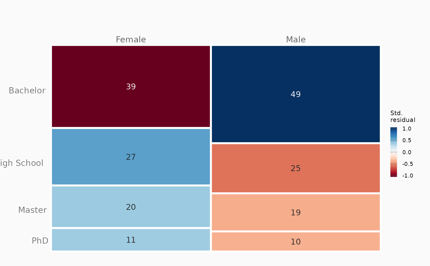 #>
#> === MOSAIC ANALYSIS RESULTS ===
#> Variables: gender × education
#> Minimum count threshold: 10
#> Test used: Chi-square test
#> Percentages based on: total
#>
#> CONSOLIDATED FREQUENCY TABLE
#> ===========================
#> # A tibble: 9 × 7
#> Variable Type Bachelor `High School` Master PhD Total
#> <chr> <chr> <dbl> <dbl> <dbl> <dbl> <dbl>
#> 1 "Female" Observed 39 27 20 11 97
#> 2 "" Expected 42.7 25.2 18.9 10.2 97
#> 3 "" % (total) 19.5 13.5 10 5.5 48.5
#> 4 "Male" Observed 49 25 19 10 103
#> 5 "" Expected 45.3 26.8 20.1 10.8 103
#> 6 "" % (total) 24.5 12.5 9.5 5 51.5
#> 7 "Total" Observed 88 52 39 21 200
#> 8 "" Expected 88 52 39 21 200
#> 9 "" % (total) 44 26 19.5 10.5 100
#>
#> STANDARDIZED RESIDUALS
#> =====================
#> (Values > |2| indicate significant deviation from expected)
#> # A tibble: 2 × 5
#> Variable Bachelor `High School` Master PhD
#> <chr> <dbl> <dbl> <dbl> <dbl>
#> 1 Female -1.05 0.57 0.39 0.38
#> 2 Male 1.05 -0.57 -0.39 -0.38
#>
#> STATISTICAL SUMMARY
#> ==================
#> # A tibble: 8 × 2
#> Statistic Value
#> <chr> <chr>
#> 1 Test type Chi-square test
#> 2 Test statistic 1.108
#> 3 Degrees of freedom 3
#> 4 p-value 0.775
#> 5 Cramer's V 0.074
#> 6 Effect size negligible
#> 7 Sample size 200
#> 8 Categories removed None
#>
# Access results
results$cramers_v
#> [1] 0.07441584
results$cramers_v_interpretation
#> [1] "negligible"
results$stats_summary
#> # A tibble: 8 × 2
#> Statistic Value
#> <chr> <chr>
#> 1 Test type Chi-square test
#> 2 Test statistic 1.108
#> 3 Degrees of freedom 3
#> 4 p-value 0.775
#> 5 Cramer's V 0.074
#> 6 Effect size negligible
#> 7 Sample size 200
#> 8 Categories removed None
# \donttest{
# With row percentages and custom labels
results <- mosaic_analysis(
example_data, "gender", "education",
min_count = 5,
var1_label = "Gender",
var2_label = "Education Level",
percentage_base = "row"
)
#>
#> === MOSAIC ANALYSIS RESULTS ===
#> Variables: gender × education
#> Minimum count threshold: 10
#> Test used: Chi-square test
#> Percentages based on: total
#>
#> CONSOLIDATED FREQUENCY TABLE
#> ===========================
#> # A tibble: 9 × 7
#> Variable Type Bachelor `High School` Master PhD Total
#> <chr> <chr> <dbl> <dbl> <dbl> <dbl> <dbl>
#> 1 "Female" Observed 39 27 20 11 97
#> 2 "" Expected 42.7 25.2 18.9 10.2 97
#> 3 "" % (total) 19.5 13.5 10 5.5 48.5
#> 4 "Male" Observed 49 25 19 10 103
#> 5 "" Expected 45.3 26.8 20.1 10.8 103
#> 6 "" % (total) 24.5 12.5 9.5 5 51.5
#> 7 "Total" Observed 88 52 39 21 200
#> 8 "" Expected 88 52 39 21 200
#> 9 "" % (total) 44 26 19.5 10.5 100
#>
#> STANDARDIZED RESIDUALS
#> =====================
#> (Values > |2| indicate significant deviation from expected)
#> # A tibble: 2 × 5
#> Variable Bachelor `High School` Master PhD
#> <chr> <dbl> <dbl> <dbl> <dbl>
#> 1 Female -1.05 0.57 0.39 0.38
#> 2 Male 1.05 -0.57 -0.39 -0.38
#>
#> STATISTICAL SUMMARY
#> ==================
#> # A tibble: 8 × 2
#> Statistic Value
#> <chr> <chr>
#> 1 Test type Chi-square test
#> 2 Test statistic 1.108
#> 3 Degrees of freedom 3
#> 4 p-value 0.775
#> 5 Cramer's V 0.074
#> 6 Effect size negligible
#> 7 Sample size 200
#> 8 Categories removed None
#>
# Access results
results$cramers_v
#> [1] 0.07441584
results$cramers_v_interpretation
#> [1] "negligible"
results$stats_summary
#> # A tibble: 8 × 2
#> Statistic Value
#> <chr> <chr>
#> 1 Test type Chi-square test
#> 2 Test statistic 1.108
#> 3 Degrees of freedom 3
#> 4 p-value 0.775
#> 5 Cramer's V 0.074
#> 6 Effect size negligible
#> 7 Sample size 200
#> 8 Categories removed None
# \donttest{
# With row percentages and custom labels
results <- mosaic_analysis(
example_data, "gender", "education",
min_count = 5,
var1_label = "Gender",
var2_label = "Education Level",
percentage_base = "row"
)
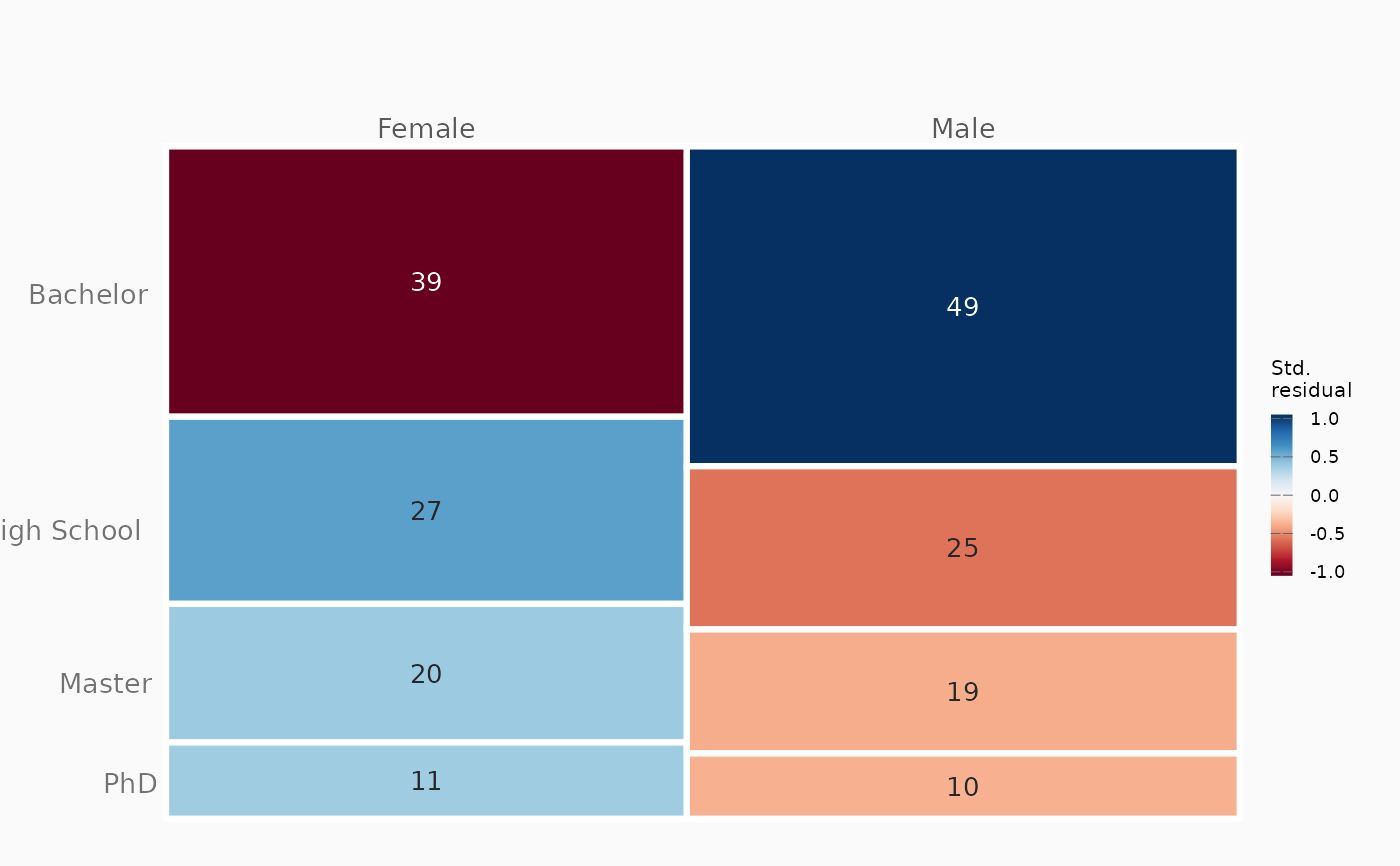 #>
#> === MOSAIC ANALYSIS RESULTS ===
#> Variables: gender × education
#> Minimum count threshold: 5
#> Test used: Chi-square test
#> Percentages based on: row
#>
#> CONSOLIDATED FREQUENCY TABLE
#> ===========================
#> # A tibble: 9 × 7
#> Variable Type Bachelor `High School` Master PhD Total
#> <chr> <chr> <dbl> <dbl> <dbl> <dbl> <dbl>
#> 1 "Female" Observed 39 27 20 11 97
#> 2 "" Expected 42.7 25.2 18.9 10.2 97
#> 3 "" % (row) 40.2 27.8 20.6 11.3 100
#> 4 "Male" Observed 49 25 19 10 103
#> 5 "" Expected 45.3 26.8 20.1 10.8 103
#> 6 "" % (row) 47.6 24.3 18.4 9.7 100
#> 7 "Total" Observed 88 52 39 21 200
#> 8 "" Expected 88 52 39 21 200
#> 9 "" % (row) 87.8 52.1 39 21 200.
#>
#> STANDARDIZED RESIDUALS
#> =====================
#> (Values > |2| indicate significant deviation from expected)
#> # A tibble: 2 × 5
#> Variable Bachelor `High School` Master PhD
#> <chr> <dbl> <dbl> <dbl> <dbl>
#> 1 Female -1.05 0.57 0.39 0.38
#> 2 Male 1.05 -0.57 -0.39 -0.38
#>
#> STATISTICAL SUMMARY
#> ==================
#> # A tibble: 8 × 2
#> Statistic Value
#> <chr> <chr>
#> 1 Test type Chi-square test
#> 2 Test statistic 1.108
#> 3 Degrees of freedom 3
#> 4 p-value 0.775
#> 5 Cramer's V 0.074
#> 6 Effect size negligible
#> 7 Sample size 200
#> 8 Categories removed None
#>
# Using Fisher's exact test for small samples
results <- mosaic_analysis(
example_data, "gender", "education",
use_fisher = TRUE,
verbose = FALSE
)
#>
#> === MOSAIC ANALYSIS RESULTS ===
#> Variables: gender × education
#> Minimum count threshold: 5
#> Test used: Chi-square test
#> Percentages based on: row
#>
#> CONSOLIDATED FREQUENCY TABLE
#> ===========================
#> # A tibble: 9 × 7
#> Variable Type Bachelor `High School` Master PhD Total
#> <chr> <chr> <dbl> <dbl> <dbl> <dbl> <dbl>
#> 1 "Female" Observed 39 27 20 11 97
#> 2 "" Expected 42.7 25.2 18.9 10.2 97
#> 3 "" % (row) 40.2 27.8 20.6 11.3 100
#> 4 "Male" Observed 49 25 19 10 103
#> 5 "" Expected 45.3 26.8 20.1 10.8 103
#> 6 "" % (row) 47.6 24.3 18.4 9.7 100
#> 7 "Total" Observed 88 52 39 21 200
#> 8 "" Expected 88 52 39 21 200
#> 9 "" % (row) 87.8 52.1 39 21 200.
#>
#> STANDARDIZED RESIDUALS
#> =====================
#> (Values > |2| indicate significant deviation from expected)
#> # A tibble: 2 × 5
#> Variable Bachelor `High School` Master PhD
#> <chr> <dbl> <dbl> <dbl> <dbl>
#> 1 Female -1.05 0.57 0.39 0.38
#> 2 Male 1.05 -0.57 -0.39 -0.38
#>
#> STATISTICAL SUMMARY
#> ==================
#> # A tibble: 8 × 2
#> Statistic Value
#> <chr> <chr>
#> 1 Test type Chi-square test
#> 2 Test statistic 1.108
#> 3 Degrees of freedom 3
#> 4 p-value 0.775
#> 5 Cramer's V 0.074
#> 6 Effect size negligible
#> 7 Sample size 200
#> 8 Categories removed None
#>
# Using Fisher's exact test for small samples
results <- mosaic_analysis(
example_data, "gender", "education",
use_fisher = TRUE,
verbose = FALSE
)
 # }
# }