Draw a temporal network — plot.dynet • Dynet

Nine views, each answering a different question.

"events": Every contact as a link drawn at the moment it fires, with actors on the vertical axis. A link leaves its source in the source's colour and arrives in the target's.
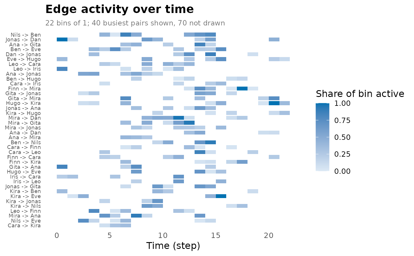
"timeline": Edge activity as an intensity heatmap, one row per pair. This is the view a static network cannot give you: it shows at a glance whether the network was busy throughout or concentrated in a few bursts.
"activity": Edges forming and dissolving over time.
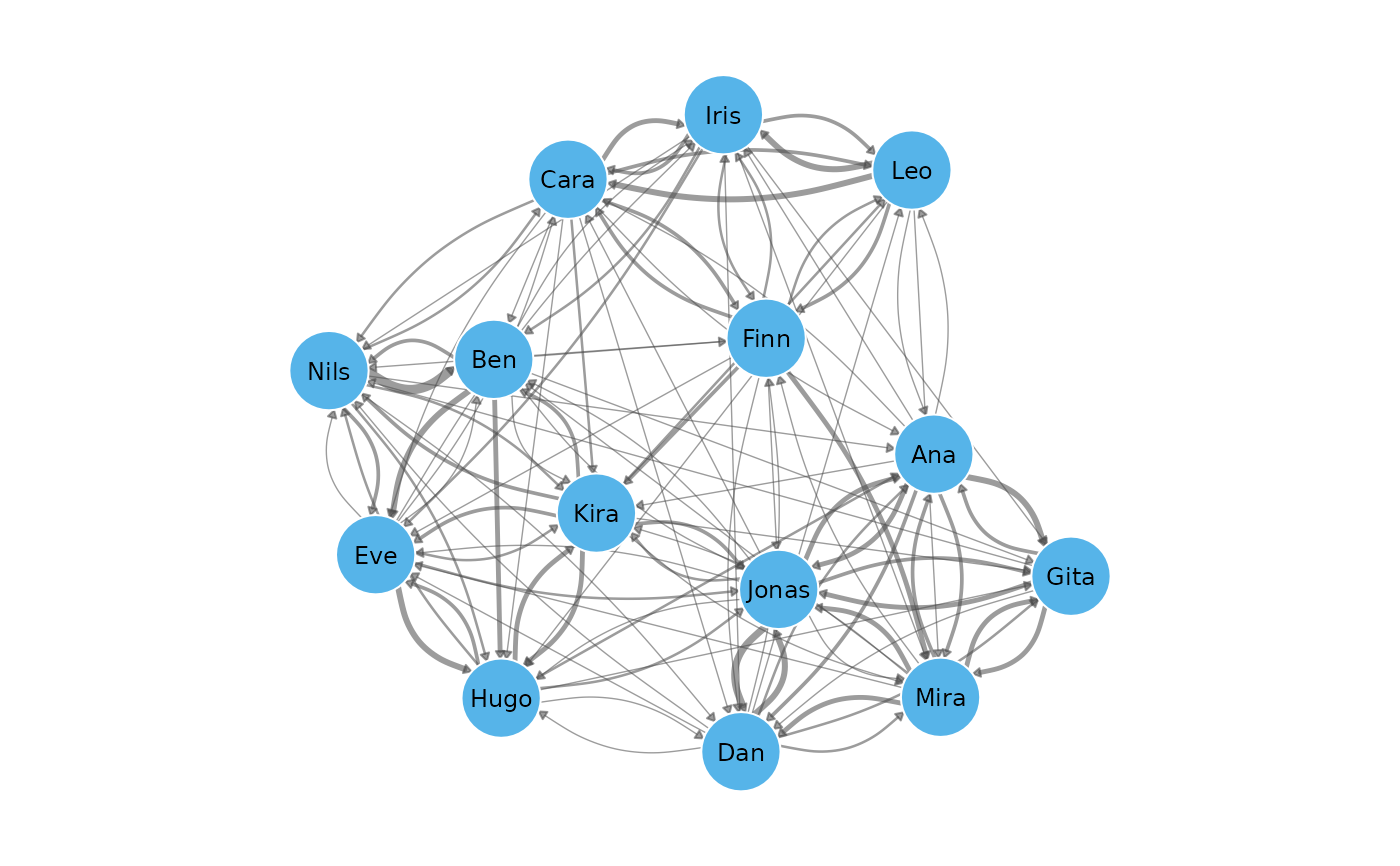
"network": The network as a node-link diagram, drawn by cograph::splot(). With no at, the whole window is flattened into one picture – useful as a reference point, and as a reminder of how much it overstates, since every tie appears simultaneous. With at, only that time bin is drawn.
"snapshots": Small multiples, one cograph::splot() per time bin, laid out on shared coordinates so positions are comparable across panels.
"layers": The multilayer view: one network per time slice, drawn as a stack of layers in which each vertex appears once per slice and is joined to its own copy in the next by an identity arc of weight omega.
"heatmap": The matrix counterpart of "layers": each slice is a tilted heatmap plane rather than a node-link diagram.
"stack": The same slices projected as a node-link stack, each vertex keeping one colour through the whole stack so it can be followed between planes.
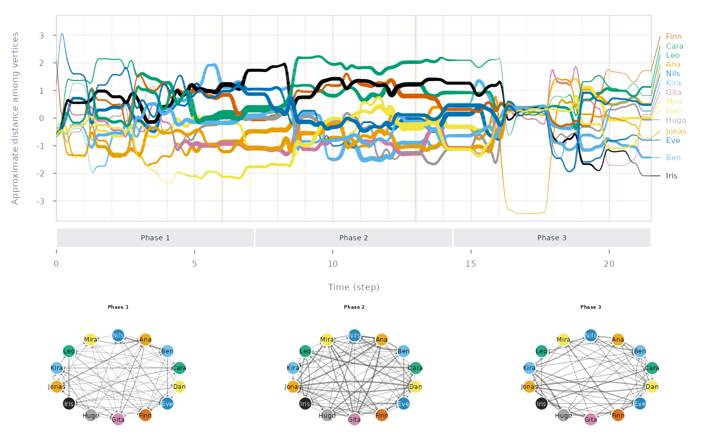
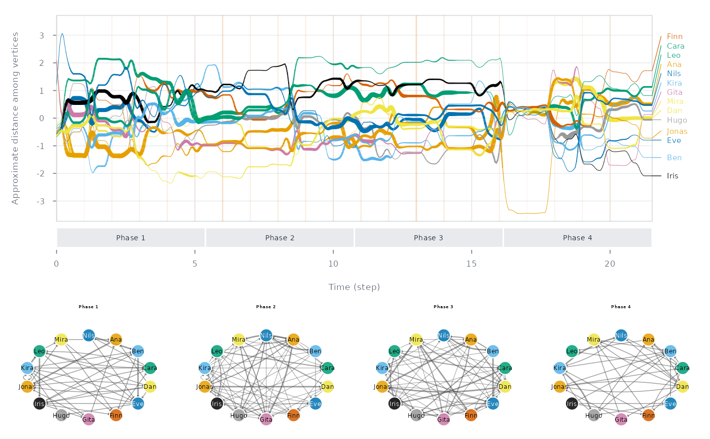
"proximity": Vertices placed on a vertical line at each time point according to how close they are in the network, and joined through time. Clusters appear as bands of lines travelling together.

All node-link rendering is cograph's. A dynet object is a cograph netobject, so cograph::splot(dn) works directly and every one of its rendering arguments is available here through ....

Usage

# S3 method for class 'dynet'
plot(
  x,
  type = c("timeline", "events", "activity", "network", "snapshots", "proximity",
    "layers", "heatmap", "stack"),
  at = NULL,
  start = NULL,
  end = NULL,
  top = 40L,
  step = NULL,
  omega = 1,
  bins = NULL,
  link = c("hook", "arc", "chevron", "wave", "bracket"),
  time = c("bin", "event", "clock"),
  aggregate = TRUE,
  nest = c("pair", "column"),
  split = 0.8,
  blend = FALSE,
  weight = TRUE,
  node_size = NULL,
  node_shape = NULL,
  node_fill = NULL,
  node_border_color = NULL,
  node_border_width = NULL,
  node_alpha = NULL,
  edge_color = NULL,
  edge_alpha = NULL,
  edge_width = NULL,
  edge_width_range = NULL,
  edge_style = NULL,
  edge_start_style = NULL,
  edge_start_length = NULL,
  curvature = NULL,
  curve_pivot = NULL,
  label_size = NULL,
  label_color = NULL,
  label_fontface = NULL,
  panels = 9L,
  measure = "degree",
  phases = NULL,
  networks = TRUE,
  events = TRUE,
  labels = TRUE,
  highlight = NULL,
  slices = 120L,
  window = NULL,
  flow = 2L,
  palette = "okabe",
  default_dist = 2,
  base_size = 12,
  style = .dyn_style(),
  ...
)

Arguments

x: A temporal network from dynet().
type: One of "timeline" (the default), "events", "activity", "network", "snapshots", "layers", "heatmap", "stack" or "proximity".
at: For "network", the time to draw. NULL draws the whole window flattened.
start, end: Window the plot to [start, end] before drawing. Either may be NULL, which keeps that side of the observed range. Every view is windowed, and an empty window is an error rather than an empty panel.
top: For the timeline, draw only the top busiest vertex pairs. Defaults to 40.
step: Width of one time bin, in the network's time unit. For "timeline" and "events" it is the bin the activity is counted in (1/24 on a network measured in days is hourly); for "layers", "heatmap" and "stack" it is the width of each slice, and at least two slices are needed, so too wide a step is an error rather than a single panel. NULL uses the construction interval.
omega: For "layers", the weight on the identity arcs carrying a vertex between adjacent slices, that is, the interlayer coupling. One non-negative number, 1 by default.
bins: Number of equal time bins for "timeline" and "events". NULL uses the network's own interval. step, a width, takes precedence when both are given.
link: Link glyph for "events": "hook" (the default), "arc", "chevron", "wave" or "bracket".
time: Time axis for "events". "bin", the default, groups onsets into equal windows and keeps duration honest, "event" gives one evenly spaced column per distinct onset, "clock" uses true positions.
aggregate: For "events", fold repeat firings of one pair inside one column into a single link, TRUE by default. Binning merges distinct onsets, and without this they stack as parallel bows carrying no extra reading.
nest: For "events", which links are fanned apart. "pair", the default, fans only links joining the same two rows in the same column; "column" fans every link sharing a column.
split: For "events", the share of each link that keeps its source colour before switching to its target's, so direction reads without arrowheads. One number between 0 and 1, 0.8 by default.
blend: For "events", fade between the two endpoint colours instead of switching at a boundary. FALSE by default.
weight: For "events", scale alpha and width by how often the pair occurs across the network, so one-off links recede and habitual ones stand out. TRUE by default.
node_size, node_shape, node_fill, node_border_color, node_border_width, node_alpha: Node aesthetics, named as in cograph::splot(). NULL uses the view's own default. They are honoured by the "network", "snapshots" and "events" views; the "layers", "heatmap", "stack" and "proximity" views take their renderer's own arguments through ....
edge_color, edge_alpha, edge_width, edge_width_range, edge_style: Link aesthetics, named as in cograph::splot(). An edge_color overrides the source-to-target colour run with one colour.
edge_start_style, edge_start_length: How the origin of each link is marked, named as in cograph::splot(). For "events" the defaults follow cograph's TNA styling: the first 0.2 of every link, from its source, is "dotted"; "dashed" is also accepted and "solid" turns the mark off. edge_start_length is a share between 0 and 0.5.
curvature, curve_pivot: Bow geometry, as in cograph::splot(). curvature is the base bow as a fraction of the column gap and 0 draws straight links; curve_pivot slides where the bow peaks.
label_size, label_color, label_fontface: Axis label aesthetics, named as in cograph::splot().
panels: For snapshots, the maximum number of panels to draw, 9 by default. Bins are sampled evenly across the window and the choice is reported.
measure: For the proximity view, the node-level measure that line thickness follows, "degree" by default. Any measure centrality_series() accepts at snapshot scope; the temporal-scope-only measures "reach" and "reach_count" are not available here, because the view redraws the measure over many short slices.
phases: For the proximity view, how many phases to split the window into for the network panels. NULL uses the network's sessions when it has them and three phases otherwise.
networks: Whether the proximity view draws a network panel per phase, TRUE by default.
events: Whether the proximity view marks the times edges formed, TRUE by default.
labels: Whether vertices are named, TRUE by default: beside each node in the "network", "snapshots", "layers" and "stack" views, and at the right-hand end of each line in the proximity view in place of a legend. The "timeline", "events", "activity" and "heatmap" views name their axes rather than their vertices and ignore it. FALSE is the readable choice for a network of more than a few dozen vertices.
highlight: Vertex names to draw in colour in the proximity view, with the rest in grey. NULL, the default, colours every vertex.
slices: How many times the proximity view measures the network across the window, 120 by default. Smoothness comes from measuring often, never from interpolation. NULL measures once per time bin, and anything else must be at least two.
window: Width of each proximity slice. NULL uses a sixth of the observation window, or the bin width if that is wider: scaling is only meaningful on a slice whose network is connected, and over one narrow bin most vertices are isolated.
flow: How many corner-cutting passes round each proximity line, 2 by default. Rounding only ever takes convex combinations of measurements, so it softens the joints without letting the curve overshoot one. 0 leaves them sharp.
palette: Colours for vertices and lines: "okabe" (the default, nine colour-blind safe colours, recycled), "extended" (hue varied with lightness, about twelve distinct), "many" (packed for separation, any number, not colour-blind safe), your own vector of colours, or a function of n returning n colours.
default_dist: Distance assumed between vertices with no path between them, in the proximity view. 2 by default.
base_size: Base font size for the "timeline", "events" and "activity" views, 12 by default. The "heatmap" view is also a ggplot but is sized by its own renderer.
style: Style constants for the proximity view's base-graphics panel: a list holding cex, grid, background, grid_color, axis_color, text_color and frame_color. The default is the package's own.
...: Passed to the renderer the chosen view uses: cograph::splot() for "network", "snapshots" and "proximity", cograph::plot_mlna() for "layers", cograph::plot_ml_heatmap() for "heatmap" and cograph::plot_temporal() for "stack". The remaining views take no further drawing arguments, and a name no view can read is an error rather than a silently ignored argument.

Value

For "timeline", "events", "activity" and "heatmap", a ggplot object, which prints itself when the call is not assigned. For "network", "snapshots", "layers", "stack" and "proximity", the figure is drawn on the current device and the network is returned invisibly – x itself, or the windowed network when start or end was given.

Details

The node-link views set a few of cograph::splot()'s defaults before handing over: they draw no edge labels and no edge-colour legend (legend_edge_colors = FALSE, against cograph::splot()'s own TRUE), colour edges a neutral grey, and size nodes and arrowheads from the vertex count. Naming any of those through ... overrides it.

Failures are classed conditions. dynet_bad_input covers every malformed argument, dynet_unknown_plot_arg a name in ... no view can read, dynet_bad_palette an unusable palette, and dynet_empty_result a window, an at or a step that leaves nothing to draw. The proximity view adds dynet_unknown_measure and dynet_needs_directed. With cograph absent, the node-link views raise dynet_needs_cograph and the "layers", "heatmap" and "stack" views dynet_missing_package.

References

Okabe, M., & Ito, K. (2008). Color universal design: how to make figures and presentations that are friendly to colorblind people.

Chaikin, G. M. (1974). An algorithm for high-speed curve generation. Computer Graphics and Image Processing, 3(4), 346-349.

Examples

dn <- dynet(school_contacts)
plot(dn)

plot(dn, type = "proximity")

plot(dn, type = "proximity", measure = "betweenness", phases = 4)

plot(dn, type = "network", node_fill = "#56B4E9")