animate() displays changes in a temporal network across
successive measurement windows. This article illustrates its use with
simulated classroom contacts and a MOOC discussion forum. The arguments
start, end, step, and
window define the measurement grid. GIF output requires
gifski; MP4 and WebM output require av.
Data
school_contacts contains 240 simulated face-to-face
contacts among fourteen students, with onset and termination times. The
constructor recognises its endpoint and interval columns
automatically.
library(Dynet)
dn <- dynet(school_contacts)
dn
#> # Temporal network (interval format, directed) | a cograph netobject
#> # 14 vertices | 240 edge spells | 110 distinct pairs
#> # observed from 0 to 21.52 step, binned every 1
#>
#>   from   to start  end duration weight
#>  Jonas  Dan  0.00 1.10     1.10      1
#>   Gita  Ana  0.14 0.98     0.84      1
#>    Leo Mira  0.15 0.42     0.27      1
#>    Leo Iris  0.15 0.96     0.81      1
#>   Kira  Ben  0.33 0.69     0.36      1
#>    Leo Iris  0.38 0.50     0.12      1
#> # 234 more spells. summary() describes the network; plot() draws it.
The bins
snapshots() lists the connections represented in each
animation window. Here, step = 2 places measurements two
time units apart, and window = 4 includes connections
active at any point within each four-unit interval.
bins <- snapshots(dn, step = 2, window = 4)
summary(bins)
#>    time ties nodes weight
#> 1     0   29    14     31
#> 2     2   33    14     39
#> 3     4   50    14     61
#> 4     6   54    14     69
#> 5     8   45    14     59
#> 6    10   54    14     76
#> 7    12   51    14     70
#> 8    14   40    14     50
#> 9    16   24    14     25
#> 10   18   25    14     25
#> 11   20   17    14     17
The grid contains eleven overlapping windows. Connected-pair counts increase from 29 in the first window to 54 in the windows beginning at times 6 and 10, then decrease to seventeen in the final window. Connections displayed together within a window need not be active simultaneously.
The animation
file specifies the output path, and its extension
selects the encoder: .gif, .mp4, or
.webm. The returned tidy table describes each measurement
bin.
film <- animate(dn, step = 2, window = 4, file = "animating_files/classroom.gif")
film
#> # Animation of 11 bins in 66 frames at 12 fps | spring layout | gif | time in step
#> # animating_files/classroom.gif
#>  bin frame time window_start window_end nodes idle ties forming dissolving
#>    1     1    0            0          4    14    0   29      NA         10
#>    2     7    2            2          6    14    0   33      14          9
#>    3    13    4            4          8    14    0   50      26          9
#>    4    19    6            6         10    14    0   54      13         20
#>    5    25    8            8         12    14    0   45      11         11
#>    6    31   10           10         14    14    0   54      20         12
#>    7    37   12           12         16    14    0   51       9         15
#>    8    43   14           14         18    14    0   40       4         25
#>    9    49   16           16         20    14    0   24       9          9
#>   10    55   18           18         22    14    0   25      10          8
#>   11    61   20           20         24    14    0   17       0         NA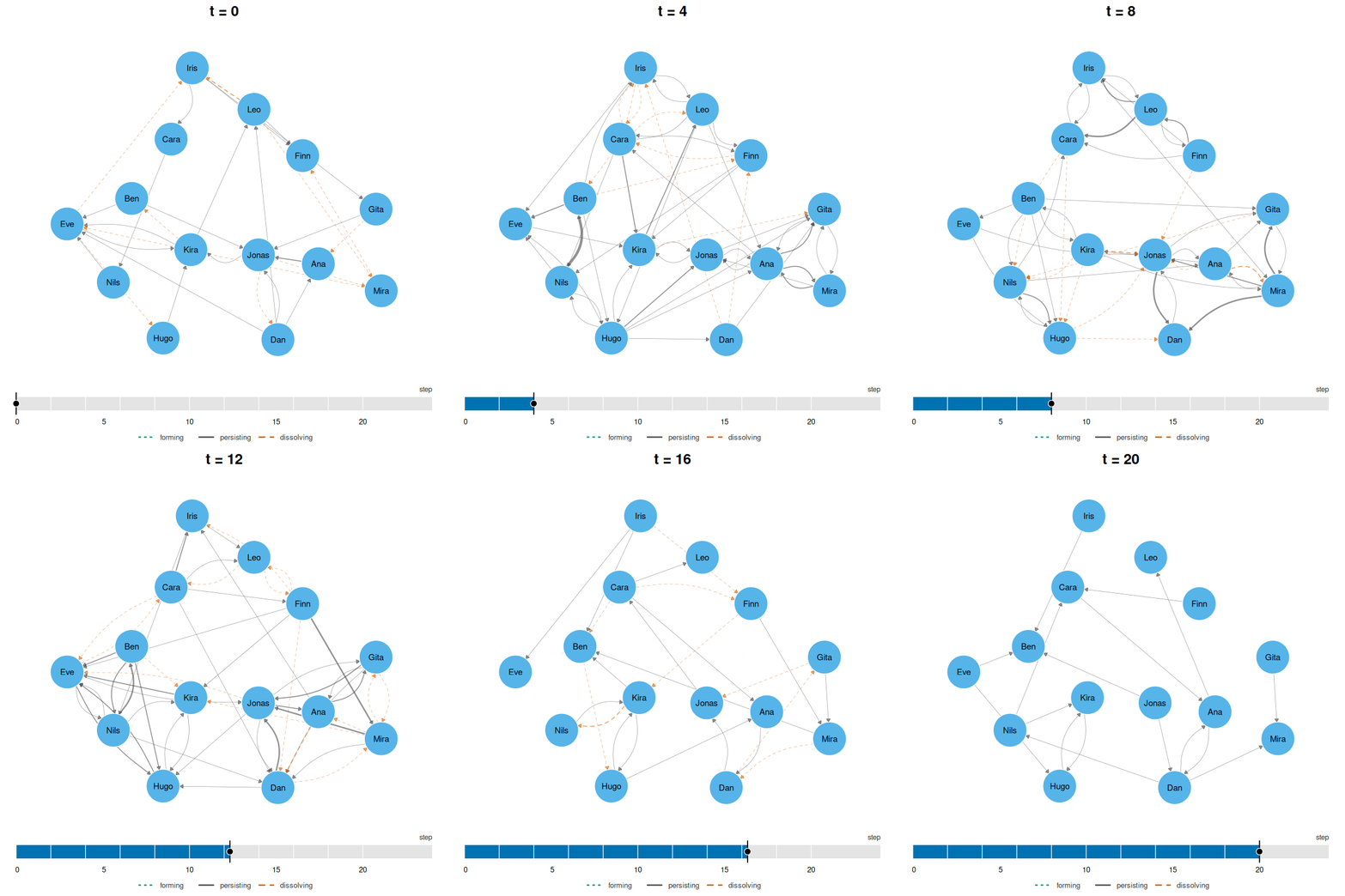
ties records the connected-pair count, matching the
corresponding snapshot. forming counts pairs present in the
current bin but absent from the preceding bin. dissolving
counts pairs present in the current bin but absent from the next. The
first bin has no predecessor and the last has no successor, so these
comparisons are NA at the respective boundaries. The bin
beginning at time 4 contains fifty pairs, of which 26 were absent from
the preceding bin and nine are absent from the next.
Forming ties are dotted and green, persisting ties are solid and grey, and dissolving ties are dashed and vermilion. Line type therefore distinguishes states as well as colour. Tie width represents weight on a common scale across frames. These states describe changes between snapshots, rather than individual spell onsets and terminations.
By default, each bin contributes six frames through
tween = 6. Forming ties fade in and dissolving ties fade
out during transitions, while a timeline marks the current interval.
summary(film)
#>   bins frames fps seconds tween  ease layout format measure first_time
#> 1   11     66  12     5.5     6 dwell spring    gif    <NA>          0
#>   last_time min_ties max_ties  turnover                          file
#> 1        20       17       54 0.3074074 animating_files/classroom.gif
Eleven bins produce 66 frames, lasting 5.5 seconds at twelve frames
per second. turnover is the median proportion of a bin’s
connections that were absent from the preceding bin; it is 0.31
here.
Vertex size
Setting measure to a snapshot centrality name scales
vertex area by the value computed within each bin. A common scale is
used throughout the animation.
per_bin <- animate(dn, step = 2, window = 4, measure = "degree",
                   file = "animating_files/classroom-degree.gif")
summary(per_bin)
#>   bins frames fps seconds tween  ease layout format measure first_time
#> 1   11     66  12     5.5     6 dwell spring    gif  degree          0
#>   last_time min_ties max_ties  turnover                                 file
#> 1        20       17       54 0.3074074 animating_files/classroom-degree.gif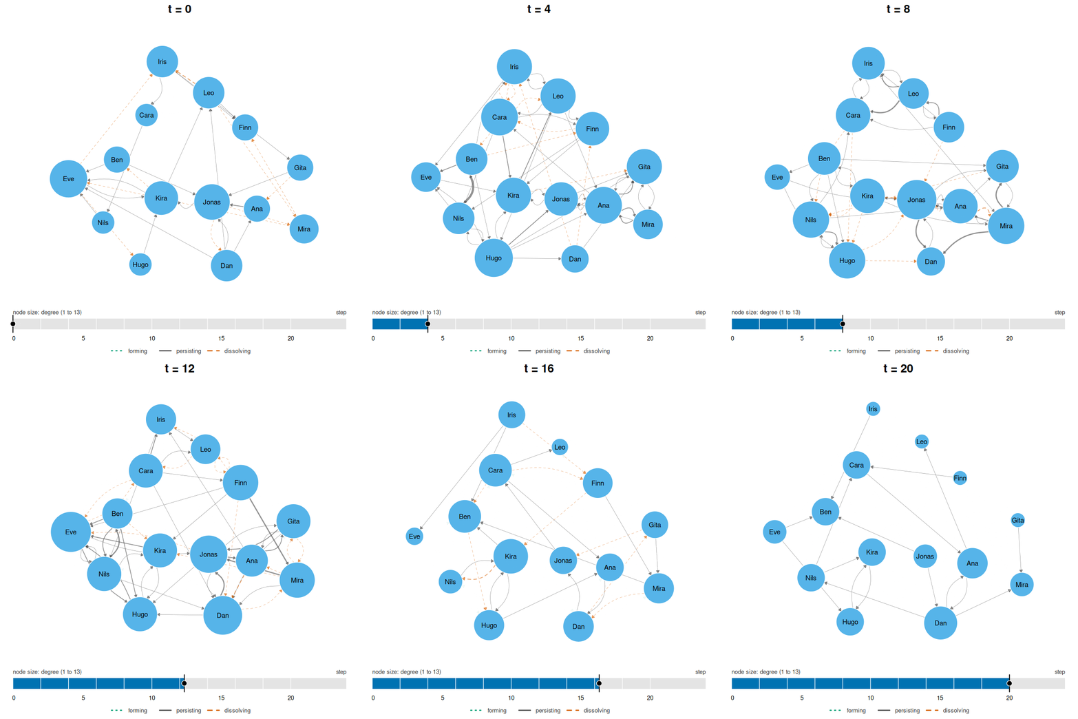
With measure = "degree", changing vertex sizes show
changes in direct connectivity. Alternatively, supply a whole-period
centrality result to keep vertex sizes constant while ties change.
whole <- centrality_series(dn, measure = "degree", window = "all")
print(whole, n = 14)
#> # Degree (node-level)
#> # 14 vertices | 1 time points, 21.52 per bin | time in step
#>  time  node measure value
#>     0   Ana  degree    16
#>     0   Ben  degree    15
#>     0  Cara  degree    17
#>     0   Dan  degree    18
#>     0   Eve  degree    17
#>     0  Finn  degree    15
#>     0  Gita  degree    13
#>     0  Hugo  degree    15
#>     0  Iris  degree    15
#>     0 Jonas  degree    18
#>     0  Kira  degree    17
#>     0   Leo  degree    12
#>     0  Mira  degree    16
#>     0  Nils  degree    16
fixed <- animate(dn, step = 2, window = 4, measure = whole,
                 file = "animating_files/classroom-whole.gif")
summary(fixed)
#>   bins frames fps seconds tween  ease layout format
#> 1   11     66  12     5.5     6 dwell spring    gif
#>                        measure first_time last_time min_ties max_ties  turnover
#> 1 Degree over the whole period          0        20       17       54 0.3074074
#>                                  file
#> 1 animating_files/classroom-whole.gif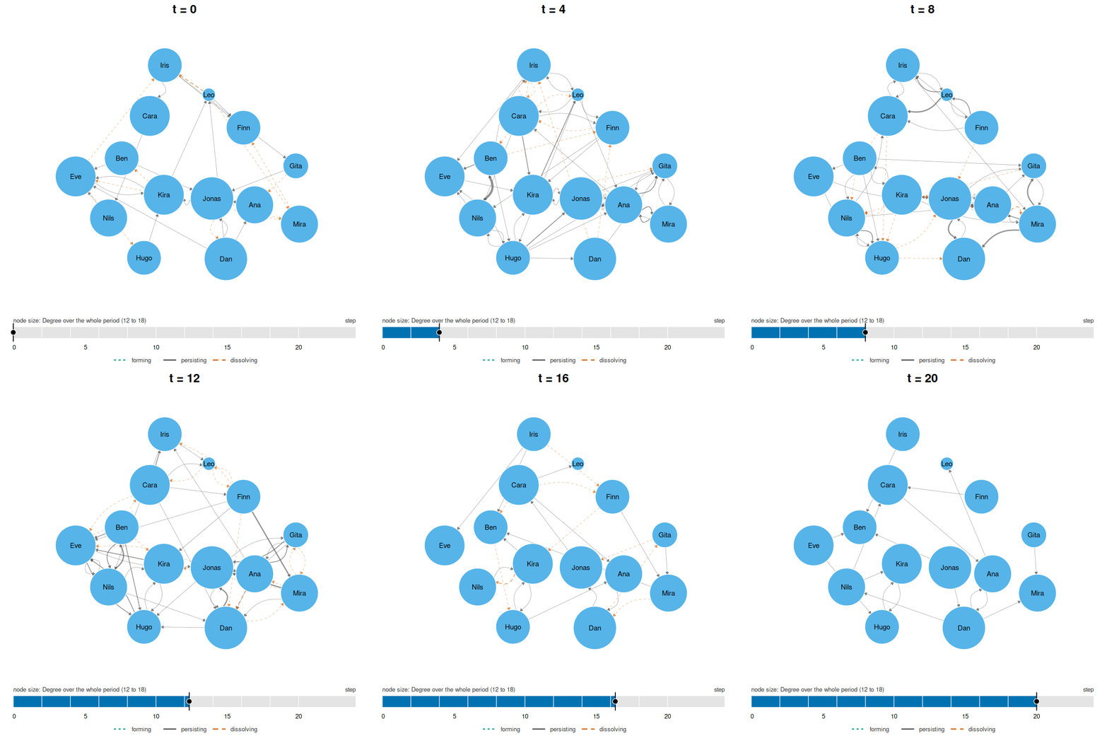
Dan and Jonas have whole-period total degree eighteen, compared with twelve for Leo, so they appear larger in every frame. Because the network is directed and degree sums incoming and outgoing connections by default, these values do not necessarily equal the number of distinct partners.
Layout
The default layout = "spring" computes positions from
the union of connections across bins and reuses them in every frame.
Fixed positions make changes in connections easier to compare.
With layout = "relaxed", positions are recalculated for
each bin using the preceding layout as a starting point and a positional
constraint. max_displacement, which defaults to 0.08 layout
units, limits movement between bins.
drift <- animate(dn, step = 2, window = 4, measure = "degree",
                 layout = "relaxed",
                 file = "animating_files/classroom-relaxed.mp4")
summary(drift)
#>   bins frames fps seconds tween  ease  layout format measure first_time
#> 1   11     66  12     5.5     6 dwell relaxed    mp4  degree          0
#>   last_time min_ties max_ties  turnover                                  file
#> 1        20       17       54 0.3074074 animating_files/classroom-relaxed.mp4
A relaxed layout can display changes in local grouping, although movement itself is part of the visualisation rather than an observed participant trajectory. A fixed layout provides stable reference positions across time.
Presence
The MOOC forum data contain reply timestamps and discussion identifiers. Threaded construction represents each reply relationship as active from its posting time until the last retained interaction in its discussion.
The following call supplies participant attributes through
nodes and uses experience level for vertex colours through
groups. min_thread_posts = 2 excludes
discussions with fewer than two retained posts after self-reply removal.
induce_subgraph() then selects participants with
whole-period total degree greater than twenty.
dn_full <- dynet(mooc_posts, from = "sender", to = "receiver",
                 time = "timestamp", thread = "discussion",
                 nodes = mooc_people, time_unit = "days",
                 groups = "expert_level", min_thread_posts = 2)
forum <- induce_subgraph(dn_full, degree > 20)
forum
#> # Temporal network (threaded format, directed) | a cograph netobject
#> # 45 vertices | 686 edge spells | 428 distinct pairs
#> # observed from 0.1138889 to 72.01111 days, binned every 1
#> # vertex attributes: experience, expert_level, groups
#>
#>  from  to     start      end duration weight
#>   219 444 0.1138889 69.47778 69.36389      1
#>   310 444 0.1680556 68.38681 68.21875      1
#>    19 310 0.2784722 14.10486 13.82639      1
#>    19 444 0.2909722 69.47778 69.18681      1
#>    30 444 0.8791667 69.47778 68.59861      1
#>    30 444 0.8819444 68.38681 67.50486      1
#>                                                                     thread
#>                         Most important change for your school or district?
#>                                  Submitting Questions for the Expert Panel
#>  How important is teacher training in a digital learning transition phase?
#>                         Most important change for your school or district?
#>                         Most important change for your school or district?
#>                                  Submitting Questions for the Expert Panel
#> # 680 more spells. summary() describes the network; plot() draws it.
The subgraph contains 45 vertices, 686 spells, and 428 distinct ordered pairs, spanning days 0.11–72.01. The data do not directly record enrolment or departure, so vertices are initially treated as eligible throughout observation.
set_vertex_spells(..., "ties") derives an activity
period from each participant’s first spell onset to their last spell
termination. This is an inferred participation period, not a recorded
arrival or departure time.
forum <- set_vertex_spells(forum, "ties")
spans <- as.data.frame(forum, what = "vertex_spells")
head(spans)
#>   vertex_spell node     start      end duration instant session onset_censored
#> 1            1    1  4.120139 71.40625 67.28611   FALSE    <NA>          FALSE
#> 2            2  100 12.842361 70.53958 57.69722   FALSE    <NA>          FALSE
#> 3            3   11  4.061806 71.43819 67.37639   FALSE    <NA>          FALSE
#> 4            4  116  3.164583 70.53958 67.37500   FALSE    <NA>          FALSE
#> 5            5   13 18.147222 72.01111 53.86389   FALSE    <NA>          FALSE
#> 6            6  137 11.107639 69.47778 58.37014   FALSE    <NA>          FALSE
#>   terminus_censored
#> 1             FALSE
#> 2             FALSE
#> 3             FALSE
#> 4             FALSE
#> 5             FALSE
#> 6             FALSE
The derived activity periods extend from day 4.12 to 71.41 for participant 1 and from day 18.15 to 72.01 for participant 13.
absent controls the display of vertices outside their
declared activity periods. The default "fade" retains their
positions at quarter opacity. "away" moves them out of view
while absent, with animated transitions at arrival and departure.
The following animation uses seven-day windows beginning every two
days. labels = FALSE omits participant identifiers, and
palette supplies colours for the three experience
levels.
arrivals <- animate(forum, start = 0, end = 70, step = 2, window = 7,
                    measure = "degree", absent = "away", labels = FALSE,
                    palette = c("#E69F00", "#56B4E9", "#CC79A7"),
                    file = "animating_files/forum.mp4")
print(arrivals, n = 36)
#> # Animation of 36 bins in 216 frames at 12 fps | spring layout | mp4 | time in days
#> # node size follows degree
#> # animating_files/forum.mp4
#>  bin frame time window_start window_end nodes idle ties forming dissolving
#>    1     1    0            0          7    29    0   53      NA          0
#>    2     7    2            2          9    29    0   59       6          0
#>    3    13    4            4         11    29    0   66       7          0
#>    4    19    6            6         13    37    0   81      15          4
#>    5    25    8            8         15    38    0   95      18          0
#>    6    31   10           10         17    39    0  101       6          6
#>    7    37   12           12         19    41    0  113      18          0
#>    8    43   14           14         21    41    0  131      18          9
#>    9    49   16           16         23    41    0  140      18         13
#>   10    55   18           18         25    42    0  134       7          3
#>   11    61   20           20         27    43    1  143      12          3
#>   12    67   22           22         29    45    1  154      14         13
#>   13    73   24           24         31    45    1  158      17          1
#>   14    79   26           26         33    45    1  180      23          5
#>   15    85   28           28         35    45    2  195      20         10
#>   16    91   30           30         37    45    2  201      16         21
#>   17    97   32           32         39    45    2  193      13         13
#>   18   103   34           34         41    44    3  186       6          6
#>   19   109   36           36         43    44    3  195      15          2
#>   20   115   38           38         45    44    3  196       3          5
#>   21   121   40           40         47    44    2  229      38         12
#>   22   127   42           42         49    44    2  242      25          6
#>   23   133   44           44         51    44    0  275      39          4
#>   24   139   46           46         53    44    0  276       5          4
#>   25   145   48           48         55    44    0  276       4         27
#>   26   151   50           50         57    44    0  251       2         34
#>   27   157   52           52         59    44    0  220       3         18
#>   28   163   54           54         61    44    0  208       6          9
#>   29   169   56           56         63    44    0  207       8          3
#>   30   175   58           58         65    44    0  204       0         25
#>   31   181   60           60         67    44    0  181       2         22
#>   32   187   62           62         69    44    0  160       1          7
#>   33   193   64           64         71    44    0  160       7          1
#>   34   199   66           66         73    44    0  164       5          7
#>   35   205   68           68         75    44    0  157       0         87
#>   36   211   70           70         77    34    0   70       0         NA
nodes counts participants eligible within each window:
29 in the first window, 45 in the window beginning on day 22, and 44 in
the window beginning on day 34. idle counts eligible
participants without a connection in the window and ranges from zero to
three. Connected-pair counts rise from 53 in the first window to 276 in
the windows beginning on days 46 and 48, then decrease to seventy in the
last.
summary(arrivals)
#>   bins frames fps seconds tween  ease layout format measure first_time
#> 1   36    216  12      18     6 dwell spring    mp4  degree          0
#>   last_time min_ties max_ties   turnover                      file
#> 1        70       53      276 0.06735751 animating_files/forum.mp4
The 36 bins produce 216 frames and an eighteen-second animation. Median turnover is 0.07.
Smoothing
Both the measurement grid and the transition settings affect
continuity between frames. Non-overlapping windows
(window = step) represent successive intervals. Overlapping
windows (window > step) share observations, which can
make changes appear more gradual. Changing the window alters the
underlying snapshots, not just their presentation.
The following call uses non-overlapping two-day windows.
tiled <- animate(forum, start = 0, end = 70, step = 2, window = 2,
                 measure = "degree", absent = "away", labels = FALSE,
                 palette = c("#E69F00", "#56B4E9", "#CC79A7"),
                 file = "animating_files/forum-tiled.mp4")
print(tiled, n = 6)
#> # Animation of 36 bins in 216 frames at 12 fps | spring layout | mp4 | time in days
#> # node size follows degree
#> # animating_files/forum-tiled.mp4
#>  bin frame time window_start window_end nodes idle ties forming dissolving
#>    1     1    0            0          2     7    0   10      NA          0
#>    2     7    2            2          4    14    0   22      12          0
#>    3    13    4            4          6    29    0   44      22          0
#>    4    19    6            6          8    29    0   58      14          4
#>    5    25    8            8         10    29    1   56       2          0
#>    6    31   10           10         12    34    1   71      15          6
#> # 30 more bins.
summary(tiled)
#>   bins frames fps seconds tween  ease layout format measure first_time
#> 1   36    216  12      18     6 dwell spring    mp4  degree          0
#>   last_time min_ties max_ties   turnover                            file
#> 1        70       10      242 0.09504132 animating_files/forum-tiled.mp4
The first two-day window contains seven eligible participants and ten connected pairs, compared with 29 participants and 53 pairs in the first seven-day window. Median turnover increases from 0.07 to 0.10. The classroom example has turnover 0.31, but the datasets and grids differ, so these values are descriptive rather than a controlled comparison.
ease controls transitions between the selected
snapshots. The default "dwell" holds each bin before
transitioning. "continuous" interpolates positions using a
spline (Catmull and Rom, 1974) and uses linear fades without a
stationary interval.
flowing <- animate(forum, start = 0, end = 70, step = 2, window = 7,
                   measure = "degree", absent = "away", labels = FALSE,
                   layout = "relaxed", ease = "continuous",
                   palette = c("#E69F00", "#56B4E9", "#CC79A7"),
                   file = "animating_files/forum-continuous.mp4")
summary(flowing)
#>   bins frames fps seconds tween       ease  layout format measure first_time
#> 1   36    216  12      18     6 continuous relaxed    mp4  degree          0
#>   last_time min_ties max_ties   turnover                                 file
#> 1        70       53      276 0.06735751 animating_files/forum-continuous.mp4
Combining a relaxed layout with continuous easing produces gradual movement. Intermediate frames interpolate between snapshots and should not be interpreted as separately measured network states.
Choosing the arguments
| Argument | Value | Interpretation |
|---|---|---|
layout |
"spring" |
Fixed vertex positions across bins |
"relaxed" |
Positions adapt to each snapshot with constrained movement | |
measure |
A snapshot measure name | Vertex area represents centrality within each bin |
| A whole-period result | Vertex area remains fixed at the supplied value | |
absent |
"fade" |
Absent vertices remain visible at reduced opacity |
"away" |
Absent vertices move out of view | |
window |
Equal to step
|
Non-overlapping measurement intervals |
Larger than step
|
Overlapping measurement intervals | |
ease |
"dwell" |
Each snapshot is held before transition |
"continuous" |
Continuous interpolation between snapshots | |
file |
.gif |
GIF output using gifski
|
.mp4 or .webm
|
Video output using av
|